Adaptive Linear Prediction

Defining a Wave Form

Here two time segments are defined from 0 to 6 seconds in steps of 1/40 of a second.

time1 = 0:0.025:4;      % from 0 to 4 seconds
time2 = 4.025:0.025:6;  % from 4 to 6 seconds
time = [time1 time2];  % from 0 to 6 seconds

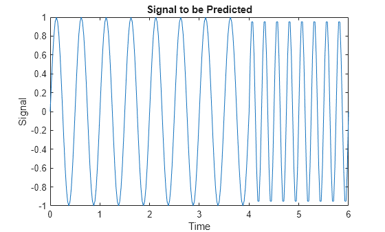
Here is a signal which starts at one frequency but then transitions to another frequency.

signal = [sin(time1*4*pi) sin(time2*8*pi)];
plot(time,signal)
xlabel('Time');
ylabel('Signal');
title('Signal to be Predicted');

Setting up the Problem for a Neural Network

The signal is then converted to a cell array. Neural Networks represent timesteps as columns of a cell array, to distinguish them from different samples at a given time, which are represented with columns of matrices.

signal = con2seq(signal);

To set up the problem we will use the first five values of the signal as initial input delay states, and the rest for inputs.

Xi = signal(1:5);
X = signal(6:end);
timex = time(6:end);

The targets are now defined to match the inputs. The network is to predict the current input, only using the last five values.

T = signal(6:end);

Creating the Linear Layer

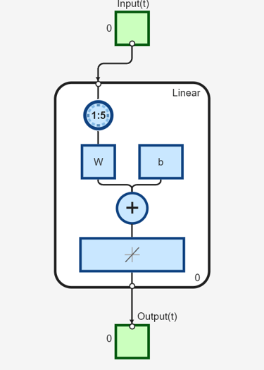
The function linearlayer creates a linear layer with a single neuron with a tap delay of the last five inputs.

net = linearlayer(1:5,0.1);
view(net)

Adapting the Linear Layer

The function adapt simulates the network on the input, while adjusting its weights and biases after each timestep in response to how closely its output matches the target. It returns the update networks, it outputs, and its errors.

[net,Y] = adapt(net,X,T,Xi);

The output signal is plotted with the targets.

figure
plot(timex,cell2mat(Y),timex,cell2mat(T),'+')
xlabel('Time');
ylabel('Output -  Target +');
title('Output and Target Signals');

The error can also be plotted.

figure
E = cell2mat(T)-cell2mat(Y);
plot(timex,E,'r')
hold off
xlabel('Time');
ylabel('Error');
title('Error Signal');

Notice how small the error is except for initial errors and the network learns the systems behavior at the beginning and after the system transition.

This example illustrated how to simulate an adaptive linear network which can predict a signal's next value from current and past values despite changes in the signals behavior.