Calibrate the SABR Model
This example shows how to use two different methods to calibrate the SABR stochastic volatility model from market implied Black volatilities. Both approaches use blackvolbysabr.
Load Market Implied Black Volatility Data
You can set up hypothetical market implied Black volatilities for European swaptions over a range of strikes before calibration. The swaptions expire in three years from the Settle date and have 10-year swaps as the underlying instrument. The rates are expressed in decimals. (Changing the units affect the numerical value and interpretation of the Alpha input parameter to the function blackvolbysabr.)
Load the market implied Black volatility data for swaptions expiring in three years.
Settle = '12-Jun-2013';
ExerciseDate = '12-Jun-2016';

MarketStrikes = [2.0 2.5 3.0 3.5 4.0 4.5 5.0]'/100;
MarketVolatilities = [45.6 41.6 37.9 36.6 37.8 39.2 40.0]'/100;
At the time of Settle, define the underlying forward rate and the at-the-money volatility.
CurrentForwardValue = MarketStrikes(4)
CurrentForwardValue =
0.0350
ATMVolatility = MarketVolatilities(4)
ATMVolatility =
0.3660
Method 1: Calibrate Alpha, Rho, and Nu Directly
The following code shows how to calibrate the Alpha, Rho, and Nu input parameters directly. The value of Beta is predetermined either by fitting historical market volatility data or by choosing a value deemed appropriate for that market [1].
Define the predetermined Beta.
Beta1 = 0.5;
After fixing the value of Beta, the parameters Alpha, Rho, and Nu are fitted directly. You can use the lsqnonlin function to generate the parameter values that minimize the squared error between the market volatilities and the volatilities computed by blackvolbysabr.
% Calibrate Alpha, Rho, and Nu.
objFun = @(X) MarketVolatilities - ...
    blackvolbysabr(X(1), Beta1, X(2), X(3), Settle, ...
    ExerciseDate, CurrentForwardValue, MarketStrikes);

X = lsqnonlin(objFun, [0.5 0 0.5], [0 -1 0], [Inf 1 Inf]);
Local minimum possible.

lsqnonlin stopped because the final change in the sum of squares relative to
its initial value is less than the value of the function tolerance.

<stopping criteria details>
Alpha1 = X(1);
Rho1 = X(2);
Nu1 = X(3);
Method 2: Calibrate Rho and Nu by Implying Alpha from At-The-Money Volatility
The following code shows how to use an alternative calibration method where the value of (Beta) is again predetermined as in Method 1.
Define the predetermined Beta.
Beta2 = 0.5;
However, after fixing the value of Beta, the parameters Alpha, Rho, and Nu are fitted directly while Alpha is implied from the market at-the-money volatility. Models calibrated using this method produce at-the-money volatilities that are equal to market quotes. This approach is widely used in swaptions, where at-the-money volatilities are quoted most frequently and are important to match. To imply Alpha from the at-the-market volatility, the following cubic polynomial is solved for Alpha and the smallest positive real root is selected [2].
![]()
where
F is the current forward value.
T is the year fraction to maturity.
To accomplish this, define an anonymous function as:
% Year fraction from Settle to option maturity
T = yearfrac(Settle, ExerciseDate, 1);

% This function solves the SABR at-the-money volatility equation as a
% polynomial of Alpha.
alpharoots = @(Rho,Nu) roots([...
    (1 - Beta2)^2*T/24/CurrentForwardValue^(2 - 2*Beta2) ...
    Rho*Beta2*Nu*T/4/CurrentForwardValue^(1 - Beta2) ...
    (1 + (2 - 3*Rho^2)*Nu^2*T/24) ...
    -ATMVolatility*CurrentForwardValue^(1 - Beta2)]);

% This function converts at-the-money volatility into Alpha by picking the
% smallest positive real root.
atmVol2SabrAlpha = @(Rho,Nu) min(real(arrayfun(@(x) ...
    x*(x>0) + realmax*(x<0 || abs(imag(x))>1e-6), alpharoots(Rho,Nu))));
The function atmVol2SabrAlpha converts at-the-money volatility into Alpha for a given set of Rho and Nu. This function is then used in the objective function to fit parameters Rho and Nu.
% Calibrate Rho and Nu (while converting at-the-money volatility into Alpha
% using atmVol2SabrAlpha).
objFun = @(X) MarketVolatilities - ...
    blackvolbysabr(atmVol2SabrAlpha(X(1), X(2)), ...
    Beta2, X(1), X(2), Settle, ExerciseDate, CurrentForwardValue, ...
    MarketStrikes);

X = lsqnonlin(objFun, [0 0.5], [-1 0], [1 Inf]);
Local minimum found.

Optimization completed because the size of the gradient is less than
the value of the optimality tolerance.

<stopping criteria details>
Rho2 = X(1);
Nu2 = X(2);
The calibrated parameter Alpha is computed using the calibrated parameters Rho and Nu.
% Obtain final Alpha from at-the-money volatility using calibrated
% parameters.
Alpha2 = atmVol2SabrAlpha(Rho2, Nu2);

% Display the calibrated parameters.
C = {Alpha1 Beta1 Rho1 Nu1;Alpha2 Beta2 Rho2 Nu2};
CalibratedPrameters = cell2table(C, ...
    'VariableNames',{'Alpha' 'Beta' 'Rho' 'Nu'}, ...
    'RowNames',{'Method 1';'Method 2'})
CalibratedPrameters=2×4 table
                 Alpha      Beta      Rho        Nu
                ________    ____    _______    _______

    Method 1    0.060277    0.5      0.2097    0.75091
    Method 2    0.058484    0.5     0.20568    0.79647
Use the Calibrated Models
The following code shows how to use the calibrated models to compute new volatilities at any strike value.
Compute volatilities for models calibrated using Method 1 and Method 2 and plot the results.
PlottingStrikes = (1.75:0.1:5.50)'/100;

% Compute volatilities for model calibrated by Method 1.
ComputedVols1 = blackvolbysabr(Alpha1, Beta1, Rho1, Nu1, Settle, ...
    ExerciseDate, CurrentForwardValue, PlottingStrikes);

% Compute volatilities for model calibrated by Method 2.
ComputedVols2 = blackvolbysabr(Alpha2, Beta2, Rho2, Nu2, Settle, ...
    ExerciseDate, CurrentForwardValue, PlottingStrikes);

figure;
plot(MarketStrikes,MarketVolatilities,'xk', ...
    PlottingStrikes,ComputedVols1,'b', ...
    PlottingStrikes,ComputedVols2,'r', ...
    CurrentForwardValue,ATMVolatility,'ok', ...
    'MarkerSize',10);
xlim([0.01 0.06]);
ylim([0.35 0.5]);
xlabel('Strike', 'FontWeight', 'bold');
ylabel('Implied Black Volatility', 'FontWeight', 'bold');
legend('Market Volatilities', 'SABR Model (Method 1)', ...
    'SABR Model (Method 2)', 'At-The-Money volatility');
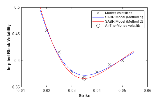
The model calibrated using Method 2 reproduces the market at-the-money volatility (marked with a circle) exactly.
References
[1] Hagan, P. S., Kumar, D., Lesniewski, A. S. and Woodward, D. E., Managing smile risk, Wilmott Magazine, 2002.
[2] West, G., "Calibration of the SABR Model in Illiquid Markets," Applied Mathematical Finance, 12(4), pp. 371–385, 2004.
See Also
blackvolbysabr | optsensbysabr | swaptionbyblk