System Identification Using Eigensystem Realization Algorithm (ERA)
This example considers a 3-degree-of-freedom (DOF) system that is excited by a series of hammer strikes. The resulting displacements are recorded by sensors. The system is proportionally damped such that the damping matrix is a linear combination of the mass and stiffness matrices. This example requires Signal Processing Toolbox™ for the section on modal analysis.
Preprocess Data
Import data for the first set of measurements. The data includes the excitation signals, response signals, time signals, and ground truth frequency-response functions. The response signal, denoted by Y1, gives the displacement of the first mass. The excitation signal consists of ten concatenated hammer impacts, and the response signal contains the corresponding displacement. The duration for each impact signal is 2.53 seconds. The excitation and response signals are corrupted with additive noise.
load modaldata XhammerMISO1 YhammerMISO1 fs;
rng('default');

% Add noise to excitation and response signals
XhammerMISO1 = XhammerMISO1 + randn(size(YhammerMISO1))/1250;
YhammerMISO1 = YhammerMISO1 + randn(size(YhammerMISO1))/1e11;

% Define outputs from function
t = (0:size(XhammerMISO1,1)-1)/fs';
X1 = 1e2*XhammerMISO1;
Y1 = 1e2*YhammerMISO1;
X0 = X1(:,1);
Y0 = Y1(:,1);
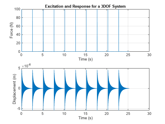
Visualize the first excitation and the response channel of the measurement.
subplot(2,1,1)
plot(t,X0)
xlabel('Time (s)')
ylabel('Force (N)')
grid on;
title('Excitation and Response for a 3DOF System')
subplot(2,1,2)
plot(t,Y0)
xlabel('Time (s)')
ylabel('Displacement (m)')
grid on;
Identify System Using ERA
Create iddata objects for estimation and validation data.
Ts = 1/fs; % sample time
estimationData = iddata(Y0(1:1000), X0(1:1000), 1/fs);
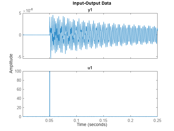
validationData = iddata(Y0(1001:2000), X0(1001:2000), 1/fs);Visualize the estimation data.
figure
plot(estimationData)
The plot of the input data shows the presence of an input delay. Remove the delay from the data.
[~,inputDelay] = max(estimationData.InputData);
estimationData = estimationData(inputDelay:end);
The era function requires data to be passed as a timetable or numeric matrix. Convert the iddata object into a timetable.
L = length(estimationData.InputData);
t = seconds(estimationData.Tstart + (0:L-1)'*Ts);
y1 = estimationData.OutputData;
tt = timetable(t,y1);
Use era to estimate a state-space model using this estimation data.
order = 6;
sys = era(tt, order, 'Feedthrough', true)
sys =
Discrete-time identified state-space model:
x(t+Ts) = A x(t) + B u(t) + K e(t)
y(t) = C x(t) + D u(t) + e(t)
A =
x1 x2 x3 x4 x5 x6
x1 0.8339 -0.5523 -0.001099 0.003053 -0.001497 0.0004633
x2 0.5523 0.8323 -0.00714 -0.001638 -0.002676 0.0008873
x3 -0.001099 0.00714 0.2293 0.9709 -0.0009399 -0.0006184
x4 -0.003053 -0.001638 -0.9709 0.2289 0.006094 -0.002101
x5 -0.001497 0.002676 -0.0009399 -0.006094 -0.5463 -0.8302
x6 -0.0004633 0.0008873 0.0006184 -0.002101 0.8302 -0.5465
B =
u1
x1 -0.001403
x2 0.0007461
x3 -0.001515
x4 -0.0001808
x5 -0.000818
x6 -0.0002384
C =
x1 x2 x3 x4 x5 x6
y1 -3.508e-07 -1.865e-07 -3.787e-07 4.52e-08 -2.045e-07 5.959e-08
D =
u1
y1 1.852e-10
K =
y1
x1 0
x2 0
x3 0
x4 0
x5 0
x6 0
Sample time: 0.00025 seconds
Parameterization:
FREE form (all coefficients in A, B, C free).
Feedthrough: yes
Disturbance component: none
Number of free coefficients: 49
Use "idssdata", "getpvec", "getcov" for parameters and their uncertainties.
Status:
Estimated using the Eigensystem Realization Algorithm
Model Properties
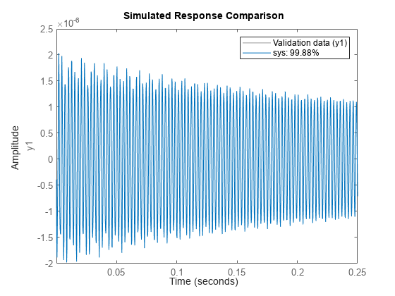
Compare the response of the estimated system with the validation data.
compare(validationData,sys);
Compare the performance of the estimated model against another state-space model estimated using ssest.
sys2 = ssest(estimationData, order, 'Feedthrough', true)sys2 =
Continuous-time identified state-space model:
dx/dt = A x(t) + B u(t) + K e(t)
y(t) = C x(t) + D u(t) + e(t)
A =
x1 x2 x3 x4 x5 x6
x1 4.985 2323 -66.74 241.3 35.31 -5.076
x2 -2341 -7.766 -300.1 11.19 11.2 25.28
x3 49.75 311 -5.616 -5360 -30.9 -15.2
x4 -270.4 -6.758 5333 -15.06 1.474 64.71
x5 -52.95 -16.58 -14.17 -34.15 3.021 8548
x6 -41.44 -15.95 -16.8 -134.7 -8674 -51.74
B =
u1
x1 -0.001651
x2 -0.02103
x3 -0.1236
x4 -0.2095
x5 -1.006
x6 0.9286
C =
x1 x2 x3 x4 x5 x6
y1 -3.244e-05 2.517e-05 1.609e-05 1.559e-05 2.731e-06 2.401e-06
D =
u1
y1 5.259e-09
K =
y1
x1 -9.881e+06
x2 8.603e+06
x3 4.435e+06
x4 2.032e+07
x5 7.865e+07
x6 -4.392e+07
Parameterization:
FREE form (all coefficients in A, B, C free).
Feedthrough: yes
Disturbance component: estimate
Number of free coefficients: 55
Use "idssdata", "getpvec", "getcov" for parameters and their uncertainties.
Status:
Estimated using SSEST on time domain data "estimationData".
Fit to estimation data: 99.6% (prediction focus)
FPE: 5.214e-17, MSE: 4.898e-17
Model Properties
compare(validationData,sys,sys2);
legend('Validation data','ERA','SSEST');
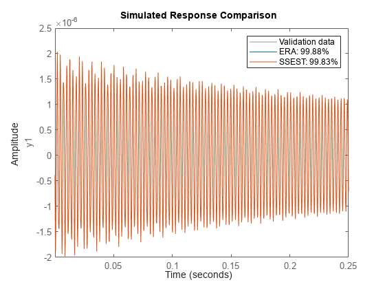
The two models have a similar fit.
Modal Analysis
Perform a modal analysis of the state-space model estimated using era by using the modalfit function from Signal Processing Toolbox. modalfit returns the damping ratios zeta and the damped natural frequencies fd.
[~,f] = modalfrf(sys);
[fd, zeta] = modalfit(sys,f,3);
View zeta.
zeta
zeta = 3×1

    0.0008
    0.0018
    0.0028
View fd.
fd
fd = 3×1
103 ×

    0.3727
    0.8525
    1.3706
Compare these results with the modes obtained from the model estimated using ssest.
[frf,f] = modalfrf(sys2);
[fd, zeta] = modalfit(sys2,f,3)
fd = 3×1
103 ×

    0.3727
    0.8525
    1.3706
zeta = 3×1

    0.0008
    0.0018
    0.0029
There is a close match between the modes obtained from modalfit for the second estimated model and those obtained for the model estimated using era.
Reduced-Order Modeling Comparison
Compare the performance of era and ssest when using a lower model order for system identification.
order = 4;
sys = era(tt, order, 'Feedthrough', true);
sys2 = ssest(estimationData, order, 'Feedthrough', true);
Compare the performance of both models as before.
compare(validationData,sys,sys2);
legend('Validation data','ERA','SSEST');
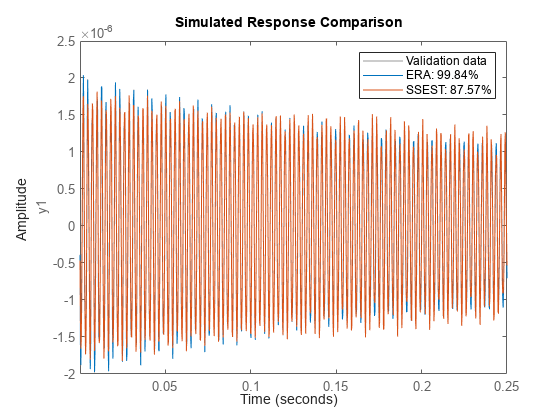
For the reduced-order model, the ERA model has a significantly better fit than the SSEST model. This result demonstrates the capability of the ERA approach in obtaining state-space models from noisy impulse response data.
See Also
era | iddata | timetable | modalfit (Signal Processing Toolbox) | modalfrf (Signal Processing Toolbox)