Deflection Analysis of Bracket
This example shows how to analyze a 3-D mechanical part under an applied load using finite element analysis (FEA) and determine the maximal deflection.
Create Structural Analysis Model
The first step in solving a linear elasticity problem is to create a structural analysis model. This model is a container that holds the geometry, structural material properties, damping parameters, body loads, boundary loads, boundary constraints, superelement interfaces, initial displacement and velocity, and mesh.
model = createpde("structural","static-solid");
Import Geometry
Import an STL file of a simple bracket model using the importGeometry function. This function reconstructs the faces, edges, and vertices of the model. It can merge some faces and edges, so the numbers can differ from those of the parent CAD model.
importGeometry(model,"BracketWithHole.stl");Plot the geometry, displaying face labels.
figure
pdegplot(model,"FaceLabels","on")
view(30,30);
title("Bracket with Face Labels")

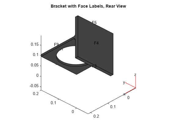
figure
pdegplot(model,"FaceLabels","on")
view(-134,-32)
title("Bracket with Face Labels, Rear View")
Specify Structural Properties of Material
Specify Young's modulus and Poisson's ratio of the material.
structuralProperties(model,"YoungsModulus",200e9, ...
                           "PoissonsRatio",0.3);
Apply Boundary Conditions and Loads
The problem has two boundary conditions: the back face (face 4) is fixed, and the front face (face 8) has an applied load. All other boundary conditions, by default, are free boundaries.
structuralBC(model,"Face",4,"Constraint","fixed");
Apply a distributed load in the negative -direction to the front face.
structuralBoundaryLoad(model,"Face",8,"SurfaceTraction",[0;0;-1e4]);
Generate Mesh
Generate and plot a mesh.
generateMesh(model);
figure
pdeplot3D(model)
title("Mesh with Quadratic Tetrahedral Elements");
Calculate Solution
Use the solve function to calculate the solution.
result = solve(model)
result =
  StaticStructuralResults with properties:

      Displacement: [1x1 FEStruct]
            Strain: [1x1 FEStruct]
            Stress: [1x1 FEStruct]
    VonMisesStress: [7780x1 double]
              Mesh: [1x1 FEMesh]
Examine Solution
Find the maximal deflection of the bracket in the -direction.
minUz = min(result.Displacement.uz);
fprintf("Maximal deflection in the z-direction is %g meters.", minUz)
Maximal deflection in the z-direction is -4.46209e-05 meters.
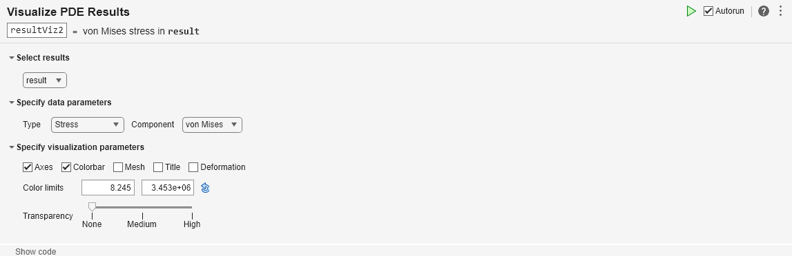
Plot Results Using Visualize PDE Results Live Editor Task
Visualize the displacement components and the von Mises stress by using the Visualize PDE Results Live Editor task. The maximal deflections are in the -direction. Because the bracket and the load are symmetric, the x-displacement and z-displacement are symmetric, and the y-displacement is antisymmetric with respect to the center line.
First, create a new live script by clicking the New Live Script button in the File section on the Home tab.

On the Live Editor tab, select Task > Visualize PDE Results. This action inserts the task into your script.

To plot the z-displacement, follow these steps. To plot the x- and y-displacements, follow the same steps, but set Component to X and Y, respectively.
In the Select results section of the task, select
resultfrom the drop-down list.In the Specify data parameters section of the task, set Type to Displacement and Component to Z.
In the Specify visualization parameters section of the task, clear the Deformation check box.
Here, the blue color represents the lowest displacement value, and the red color represents the highest displacement value. The bracket load causes face 8 to dip down, so the maximum z-displacement appears blue.


To plot the von Mises stress, in the Specify data parameters section of the task, set Type to Stress and Component to von Mises.

Plot Results at the Command Line
You also can plot the results, such as the displacement components and the von Mises stress, at the MATLAB® command line by using the pdeplot3D function.
figure
pdeplot3D(model,"ColorMapData",result.Displacement.ux)
title("x-displacement")
colormap("jet")

figure
pdeplot3D(model,"ColorMapData",result.Displacement.uy)
title("y-displacement")
colormap("jet")

figure
pdeplot3D(model,"ColorMapData",result.Displacement.uz)
title("z-displacement")
colormap("jet")

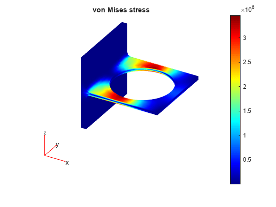
figure
pdeplot3D(model,"ColorMapData",result.VonMisesStress)
title("von Mises stress")
colormap("jet")
You can also select a web site from the following list:
Americas
- América Latina (Español)
- Canada (English)
- United States (English)
Europe
- Belgium (English)
- Denmark (English)
- Deutschland (Deutsch)
- España (Español)
- Finland (English)
- France (Français)
- Ireland (English)
- Italia (Italiano)
- Luxembourg (English)
- Netherlands (English)
- Norway (English)
- Österreich (Deutsch)
- Portugal (English)
- Sweden (English)
- Switzerland
- United Kingdom (English)