Wind Turbine High-Speed Bearing Prognosis
This example shows how to build an exponential degradation model to predict the Remaining Useful Life (RUL) of a wind turbine bearing in real time. The exponential degradation model predicts the RUL based on its parameter priors and the latest measurements (historical run-to-failure data can help estimate the model parameters priors, but they are not required). The model is able to detect the significant degradation trend in real time and updates its parameter priors when a new observation becomes available. The example follows a typical prognosis workflow: data import and exploration, feature extraction and postprocessing, feature importance ranking and fusion, model fitting and prediction, and performance analysis.
Dataset
The dataset is collected from a 2MW wind turbine high-speed shaft driven by a 20-tooth pinion gear [1]. A vibration signal of 6 seconds was acquired each day for 50 consecutive days (there are 2 measurements on March 17, which are treated as two days in this example). An inner race fault developed and caused the failure of the bearing across the 50-day period.
A compact version of the dataset is available in the toolbox. To use the compact dataset, copy the dataset to the current folder and enable its write permission.
copyfile(...
    fullfile(matlabroot, 'toolbox', 'predmaint', ...
    'predmaintdemos', 'windTurbineHighSpeedBearingPrognosis'), ...
    'WindTurbineHighSpeedBearingPrognosis-Data-main')
fileattrib(fullfile('WindTurbineHighSpeedBearingPrognosis-Data-main', '*.mat'), '+w')
The measurement time step for the compact dataset is 5 days.
timeUnit = '\times 5 day';For the full dataset, go to this link https://github.com/mathworks/WindTurbineHighSpeedBearingPrognosis-Data, download the entire repository as a zip file and save it in the same directory as this live script. Unzip the file using this command. The measurement time step for the full dataset is 1 day.
if exist('WindTurbineHighSpeedBearingPrognosis-Data-main.zip', 'file')
    unzip('WindTurbineHighSpeedBearingPrognosis-Data-main.zip')
    timeUnit = 'day';
end
The results in this example are generated from the full dataset. It is highly recommended to download the full dataset to run this example. Results generated from the compact dataset might not be meaningful.
Data Import
Create a fileEnsembleDatastore of the wind turbine data. The data contains a vibration signal and a tachometer signal. The fileEnsembleDatastore will parse the file name and extract the date information as IndependentVariables. See the helper functions in the supporting files associated with this example for more details.
hsbearing = fileEnsembleDatastore(...
    fullfile('.', 'WindTurbineHighSpeedBearingPrognosis-Data-main'), ...
    '.mat');
hsbearing.DataVariables = ["vibration", "tach"];
hsbearing.IndependentVariables = "Date";
hsbearing.SelectedVariables = ["Date", "vibration", "tach"];
hsbearing.ReadFcn = @helperReadData;
hsbearing.WriteToMemberFcn = @helperWriteToHSBearing;
tall(hsbearing)
Starting parallel pool (parpool) using the 'Processes' profile ...
Connected to parallel pool with 4 workers.

ans =

  M×3 tall table

            Date                vibration             tach
    ____________________    _________________    ______________

    11-Mar-2013 03:00:24    {292968×1 double}    {187×1 double}
    16-Mar-2013 06:56:43    {292968×1 double}    {180×1 double}
    21-Mar-2013 00:33:14    {292968×1 double}    {188×1 double}
    26-Mar-2013 01:41:50    {292968×1 double}    {180×1 double}
    31-Mar-2013 19:38:18    {292968×1 double}    {180×1 double}
    05-Apr-2013 21:35:37    {292968×1 double}    {182×1 double}
    10-Apr-2013 23:14:07    {292968×1 double}    {187×1 double}
    15-Apr-2013 22:55:24    {292968×1 double}    {167×1 double}
             :                      :                  :
             :                      :                  :
Sample rate of vibration signal is 97656 Hz.
fs = 97656; % HzData Exploration
This section explores the data in both time domain and frequency domain and seeks inspiration of what features to extract for prognosis purposes.
First visualize the vibration signals in the time domain. In this dataset, there are 50 vibration signals of 6 seconds measured in 50 consecutive days. Now plot the 50 vibration signals one after each other.
reset(hsbearing)
tstart = 0;
figure
hold on
while hasdata(hsbearing)
    data = read(hsbearing);
    v = data.vibration{1};
    t = tstart + (1:length(v))/fs;
    % Downsample the signal to reduce memory usage
    plot(t(1:10:end), v(1:10:end))
    tstart = t(end);
end
hold off
xlabel('Time (s), 6 second per day, 50 days in total')
ylabel('Acceleration (g)')
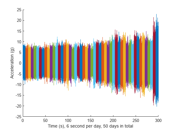
The vibration signals in time domain reveals an increasing trend of the signal impulsiveness. Indicators quantifying the impulsiveness of the signal, such as kurtosis, peak-to-peak value, crest factors etc., are potential prognostic features for this wind turbine bearing dataset [2].
On the other hand, spectral kurtosis is considered powerful tool for wind turbine prognosis in frequency domain [3]. To visualize the spectral kurtosis changes along time, plot the spectral kurtosis values as a function of frequency and the measurement day.
hsbearing.DataVariables = ["vibration", "tach", "SpectralKurtosis"];
colors = parula(50);
figure
hold on
reset(hsbearing)
day = 1;
while hasdata(hsbearing)
    data = read(hsbearing);
    data2add = table;

    % Get vibration signal and measurement date
    v = data.vibration{1};

    % Compute spectral kurtosis with window size = 128
    wc = 128;
    [SK, F] = pkurtosis(v, fs, wc);
    data2add.SpectralKurtosis = {table(F, SK)};

    % Plot the spectral kurtosis
    plot3(F, day*ones(size(F)), SK, 'Color', colors(day, :))

    % Write spectral kurtosis values
    writeToLastMemberRead(hsbearing, data2add);

    % Increment the number of days
    day = day + 1;
end
hold off
xlabel('Frequency (Hz)')
ylabel('Time (day)')
zlabel('Spectral Kurtosis')
grid on
view(-45, 30)
cbar = colorbar;
ylabel(cbar, 'Fault Severity (0 - healthy, 1 - faulty)')

Fault Severity indicated in colorbar is the measurement date normalized into 0 to 1 scale. It is observed that the spectral kurtosis value around 10 kHz gradually increases as the machine condition degrades. Statistical features of the spectral kurtosis, such as mean, standard deviation etc., will be potential indicators of the bearing degradation [3].
Feature Extraction
Based on the analysis in the previous section, a collection of statistical features derived from time-domain signal and spectral kurtosis are going to be extracted. More mathematical details about the features are provided in [2-3].
First, pre-assign the feature names in DataVariables before writing them into the fileEnsembleDatastore.
hsbearing.DataVariables = [hsbearing.DataVariables; ...
    "Mean"; "Std"; "Skewness"; "Kurtosis"; "Peak2Peak"; ...
    "RMS"; "CrestFactor"; "ShapeFactor"; "ImpulseFactor"; "MarginFactor"; "Energy"; ...
    "SKMean"; "SKStd"; "SKSkewness"; "SKKurtosis"];
Compute feature values for each ensemble member.
hsbearing.SelectedVariables = ["vibration", "SpectralKurtosis"];
reset(hsbearing)
while hasdata(hsbearing)
    data = read(hsbearing);
    v = data.vibration{1};
    SK = data.SpectralKurtosis{1}.SK;
    features = table;

    % Time Domain Features
    features.Mean = mean(v);
    features.Std = std(v);
    features.Skewness = skewness(v);
    features.Kurtosis = kurtosis(v);
    features.Peak2Peak = peak2peak(v);
    features.RMS = rms(v);
    features.CrestFactor = max(v)/features.RMS;
    features.ShapeFactor = features.RMS/mean(abs(v));
    features.ImpulseFactor = max(v)/mean(abs(v));
    features.MarginFactor = max(v)/mean(abs(v))^2;
    features.Energy = sum(v.^2);

    % Spectral Kurtosis related features
    features.SKMean = mean(SK);
    features.SKStd = std(SK);
    features.SKSkewness = skewness(SK);
    features.SKKurtosis = kurtosis(SK);

    % write the derived features to the corresponding file
    writeToLastMemberRead(hsbearing, features);
end
Select the independent variable Date and all the extracted features to construct the feature table.
hsbearing.SelectedVariables = ["Date", "Mean", "Std", "Skewness", "Kurtosis", "Peak2Peak", ...
    "RMS", "CrestFactor", "ShapeFactor", "ImpulseFactor", "MarginFactor", "Energy", ...
    "SKMean", "SKStd", "SKSkewness", "SKKurtosis"];
Since the feature table is small enough to fit in memory (50 by 15), gather the table before processing. For big data, it is recommended to perform operations in tall format until you are confident that the output is small enough to fit in memory.
featureTable = gather(tall(hsbearing));
Evaluating tall expression using the Parallel Pool 'Processes':
- Pass 1 of 1: Completed in 5.2 sec
Evaluation completed in 5.2 sec
Convert the table to timetable so that the time information is always associated with the feature values.
featureTable = table2timetable(featureTable)
featureTable=10×15 timetable
    11-Mar-2013 03:00:24    0.2139    2.0890        0.0066    3.0405    21.2170    2.0999    4.9387    1.2556     6.2009    3.7076    1.2919e+06        0.0117    0.0420    -0.7614     7.5660
    16-Mar-2013 06:56:43    0.2328    1.9755       -0.0061    3.0069    17.3361    1.9892    4.3183    1.2540     5.4151    3.4137    1.1592e+06        0.0082    0.0405     1.0274     6.4863
    21-Mar-2013 00:33:14    0.1890    2.1852    3.6700e-04    3.1416    24.8842    2.1934    6.0332    1.2592     7.5972    4.3616    1.4094e+06    8.5468e-04    0.0665    -0.3840    11.2567
    26-Mar-2013 01:41:50    0.2574    2.2293        0.0042    3.0975    23.7116    2.2441    5.3639    1.2575     6.7451    3.7797    1.4754e+06        0.0115    0.0408     0.1737     3.3943
    31-Mar-2013 19:38:18    0.2503    2.1337       -0.0037    3.0971    20.5133    2.1483    5.1751    1.2583     6.5119    3.8141    1.3521e+06        0.0156    0.0454     1.5794     7.4012
    05-Apr-2013 21:35:37    0.2118    2.2492        0.0060    3.3807    25.0880    2.2592    5.7628    1.2691     7.3138    4.1087    1.4953e+06        0.0471    0.1290     3.0512    13.2689
    10-Apr-2013 23:14:07    0.3343    2.6118        0.0022    3.8872    33.8332    2.6331    6.6096    1.2837     8.4847    4.1365    2.0312e+06        0.0616    0.1979     3.7348    17.8257
    15-Apr-2013 22:55:24    0.3521    2.0334       -0.0118    3.9380    26.4453    2.0636    6.4372    1.2869     8.2839    5.1658    1.2476e+06        0.0683    0.2072     2.9265    10.4586
    20-Apr-2013 15:13:07    0.1590    2.4311       -0.0102    4.6055    33.6220    2.4363    7.2259    1.3030     9.4153    5.0356    1.7389e+06        0.1173    0.3556     3.0585    11.7159
    25-Apr-2013 23:22:02    0.2578    2.9787        0.0259    5.4370    43.4445    2.9899    7.6824    1.3298    10.2162    4.5439    2.6189e+06        0.1656    0.5276     3.5712    16.2318
Feature Postprocessing
Extracted features are usually associated with noise. The noise with opposite trend can sometimes be harmful to the RUL prediction. In addition, one of the feature performance metrics, monotonicity, to be introduced next is not robust to noise. Therefore, a causal moving mean filter with a lag window of 5 steps is applied to the extracted features, where "causal" means no future value is used in the moving mean filtering.
variableNames = featureTable.Properties.VariableNames;
featureTableSmooth = varfun(@(x) movmean(x, [5 0]), featureTable);
featureTableSmooth.Properties.VariableNames = variableNames;
Here is an example showing the feature before and after smoothing.
figure
hold on
plot(featureTable.Date, featureTable.SKMean)
plot(featureTableSmooth.Date, featureTableSmooth.SKMean)
hold off
xlabel('Time')
ylabel('Feature Value')
legend('Before smoothing', 'After smoothing')
title('SKMean')
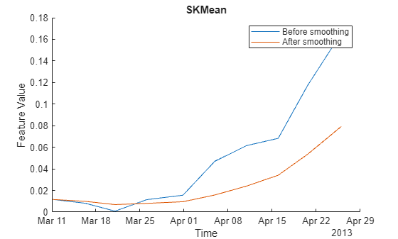
Moving mean smoothing introduces a time delay of the signal, but the delay effect can be mitigated by selecting proper threshold in the RUL prediction.
Training Data
In practice, the data of the whole lifecycle is not available when developing the prognostic algorithm, but it is reasonable to assume that some data in the early stage of the lifecycle has been collected. Hence data collected in the first 20 days (40% of the lifecycle) is treated as training data. The following feature importance ranking and fusion is only based on the training data.
breaktime = datetime(2013, 3, 27);
breakpoint = find(featureTableSmooth.Date < breaktime, 1, 'last');
trainData = featureTableSmooth(1:breakpoint, :);
Feature Importance Ranking
In this example, monotonicity proposed by [3] is used to quantify the merit of the features for prognosis purpose.
Monotonicity of th feature is computed as
where is the number of measurement points, in this case . is the number of machines monitored, in this case . is the th feature measured on th machine. , i.e. the difference of the signal .
% Since moving window smoothing is already done, set 'WindowSize' to 0 to
% turn off the smoothing within the function
featureImportance = monotonicity(trainData, 'WindowSize', 0);
helperSortedBarPlot(featureImportance, 'Monotonicity');
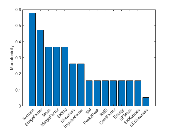
Kurtosis of the signal is the top feature based on the monotonicity.
Features with feature importance score larger than 0.3 are selected for feature fusion in the next section.
trainDataSelected = trainData(:, featureImportance{:,:}>0.3);
featureSelected = featureTableSmooth(:, featureImportance{:,:}>0.3)featureSelected=10×15 timetable
11-Mar-2013 03:00:24 0.2139 2.0890 0.0066 3.0405 21.2170 2.0999 4.9387 1.2556 6.2009 3.7076 1.2919e+06 0.0117 0.0420 -0.7614 7.5660
16-Mar-2013 06:56:43 0.2234 2.0322 2.5522e-04 3.0237 19.2765 2.0445 4.6285 1.2548 5.8080 3.5607 1.2255e+06 0.0099 0.0413 0.1330 7.0262
21-Mar-2013 00:33:14 0.2119 2.0832 2.9248e-04 3.0630 21.1458 2.0941 5.0967 1.2563 6.4044 3.8276 1.2868e+06 0.0069 0.0497 -0.0393 8.4363
26-Mar-2013 01:41:50 0.2233 2.1197 0.0013 3.0716 21.7872 2.1316 5.1635 1.2566 6.4896 3.8157 1.3340e+06 0.0080 0.0475 0.0139 7.1758
31-Mar-2013 19:38:18 0.2287 2.1225 2.7179e-04 3.0767 21.5324 2.1350 5.1658 1.2569 6.4940 3.8153 1.3376e+06 0.0096 0.0470 0.3270 7.2209
05-Apr-2013 21:35:37 0.2259 2.1437 0.0012 3.1274 22.1250 2.1557 5.2653 1.2590 6.6306 3.8642 1.3639e+06 0.0158 0.0607 0.7810 8.2289
10-Apr-2013 23:14:07 0.2459 2.2308 4.9166e-04 3.2685 24.2277 2.2445 5.5438 1.2636 7.0113 3.9357 1.4871e+06 0.0241 0.0867 1.5304 9.9389
15-Apr-2013 22:55:24 0.2658 2.2404 -4.5770e-04 3.4237 25.7459 2.2570 5.8969 1.2691 7.4894 4.2277 1.5018e+06 0.0342 0.1145 1.8469 10.6009
20-Apr-2013 15:13:07 0.2608 2.2814 -0.0022 3.6677 27.2022 2.2974 6.0957 1.2764 7.7924 4.3401 1.5568e+06 0.0536 0.1627 2.4207 10.6774
25-Apr-2013 23:22:02 0.2609 2.4063 0.0014 4.0576 30.4910 2.4217 6.4821 1.2885 8.3709 4.4674 1.7473e+06 0.0793 0.2438 2.9869 12.8170
Dimension Reduction and Feature Fusion
Principal Component Analysis (PCA) is used for dimension reduction and feature fusion in this example. Before performing PCA, it is a good practice to normalize the features into the same scale. Note that PCA coefficients and the mean and standard deviation used in normalization are obtained from training data, and applied to the entire dataset.
meanTrain = mean(trainDataSelected{:,:});
sdTrain = std(trainDataSelected{:,:});
trainDataNormalized = (trainDataSelected{:,:} - meanTrain)./sdTrain;
coef = pca(trainDataNormalized);
The mean, standard deviation and PCA coefficients are used to process the entire data set.
PCA1 = (featureSelected{:,:} - meanTrain) ./ sdTrain * coef(:, 1);
PCA2 = (featureSelected{:,:} - meanTrain) ./ sdTrain * coef(:, 2);
Visualize the data in the space of the first two principal components.
figure
numData = size(featureTable, 1);
scatter(PCA1, PCA2, [], 1:numData, 'filled')
xlabel('PCA 1')
ylabel('PCA 2')
cbar = colorbar;
ylabel(cbar, ['Time (' timeUnit ')'])
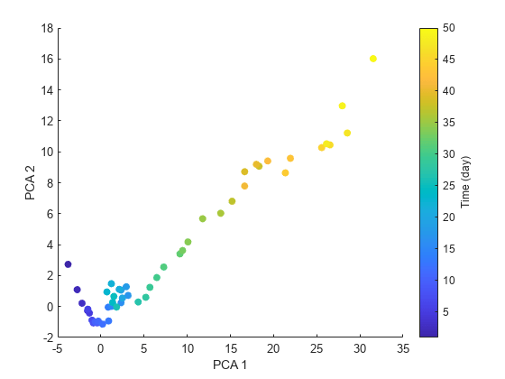
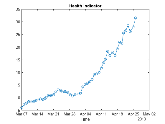
The plot indicates that the first principal component is increasing as the machine approaches to failure. Therefore, the first principal component is a promising fused health indicator.
healthIndicator = PCA1;
Visualize the health indicator.
figure
plot(featureSelected.Date, healthIndicator, '-o')
xlabel('Time')
title('Health Indicator')
Fit Exponential Degradation Models for Remaining Useful Life (RUL) Estimation
Exponential degradation model is defined as
where is the health indicator as a function of time. is the intercept term considered as a constant. and are random parameters determining the slope of the model, where is lognormal-distributed and is Gaussian-distributed. At each time step , the distribution of and is updated to the posterior based on the latest observation of . is a Gaussian white noise yielding to . The term in the exponential is to make the expectation of satisfy
.
Here an Exponential Degradation Model is fit to the health indicator extracted in the last section, and the performances is evaluated in the next section.
First shift the health indicator so that it starts from 0.
healthIndicator = healthIndicator - healthIndicator(1);
The selection of threshold is usually based on the historical records of the machine or some domain-specific knowledge. Since no historical data is available in this dataset, the last value of the health indicator is chosen as the threshold. It is recommended to choose the threshold based on the smoothed (historical) data so that the delay effect of smoothing will be partially mitigated.
threshold = healthIndicator(end);
If historical data is available, use fit method provided by exponentialDegradationModel to estimate the priors and intercept. However, historical data is not available for this wind turbine bearing dataset. The prior of the slope parameters are chosen arbitrarily with large variances () so that the model is mostly relying on the observed data. Based on , intercept is set to so that the model will start from 0 as well.
The relationship between the variation of health indicator and the variation of noise can be derived as
Here the standard deviation of the noise is assumed to cause 10% of variation of the health indicator when it is near the threshold. Therefore, the standard deviation of the noise can be represented as .
The exponential degradation model also provides a functionality to evaluate the significance of the slope. Once a significant slope of the health indicator is detected, the model will forget the previous observations and restart the estimation based on the original priors. The sensitivity of the detection algorithm can be tuned by specifying SlopeDetectionLevel. If p value is less than SlopeDetectionLevel, the slope is declared to be detected. Here SlopeDetectionLevel is set to 0.05.
Now create an exponential degradation model with the parameters discussed above.
mdl = exponentialDegradationModel(...
    'Theta', 1, ...
    'ThetaVariance', 1e6, ...
    'Beta', 1, ...
    'BetaVariance', 1e6, ...
    'Phi', -1, ...
    'NoiseVariance', (0.1*threshold/(threshold + 1))^2, ...
    'SlopeDetectionLevel', 0.05);
Use predictRUL and update methods to predict the RUL and update the parameter distribution in real time.
% Keep records at each iteration
totalDay = length(healthIndicator) - 1;
estRULs = zeros(totalDay, 1);
trueRULs = zeros(totalDay, 1);
CIRULs = zeros(totalDay, 2);
pdfRULs = cell(totalDay, 1);

% Create figures and axes for plot updating
figure
ax1 = subplot(2, 1, 1);
ax2 = subplot(2, 1, 2);

for currentDay = 1:totalDay

    % Update model parameter posterior distribution
    update(mdl, [currentDay healthIndicator(currentDay)])

    % Predict Remaining Useful Life
    [estRUL, CIRUL, pdfRUL] = predictRUL(mdl, ...
                                         [currentDay healthIndicator(currentDay)], ...
                                         threshold);
    trueRUL = totalDay - currentDay + 1;

    % Updating RUL distribution plot
    helperPlotTrend(ax1, currentDay, healthIndicator, mdl, threshold, timeUnit);
    helperPlotRUL(ax2, trueRUL, estRUL, CIRUL, pdfRUL, timeUnit)

    % Keep prediction results
    estRULs(currentDay) = estRUL;
    trueRULs(currentDay) = trueRUL;
    CIRULs(currentDay, :) = CIRUL;
    pdfRULs{currentDay} = pdfRUL;

    % Pause 0.1 seconds to make the animation visible
    pause(0.1)
end
Warning: Data does not satisfy exponential model assumption. Check model's prior parameters or try a different degradation model.
Warning: Data does not satisfy exponential model assumption. Check model's prior parameters or try a different degradation model.
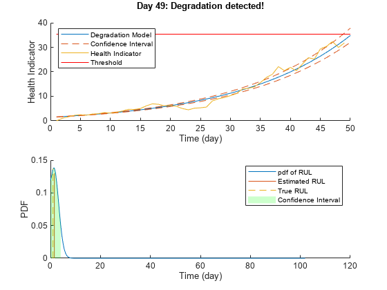
Here is the animation of the real-time RUL estimation.
Performance Analysis
- plot is used for prognostic performance analysis [5], where bound is set to 20%. The probability that the estimated RUL is between the bound of the true RUL is calculated as a performance metric of the model:
where is the estimated RUL at time , is the true RUL at time , is the estimated model parameters at time .
alpha = 0.2;
detectTime = mdl.SlopeDetectionInstant;
prob = helperAlphaLambdaPlot(alpha, trueRULs, estRULs, CIRULs, ...
    pdfRULs, detectTime, breakpoint, timeUnit);
title('\alpha-\lambda Plot')
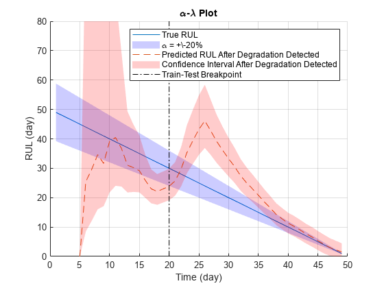
Since the preset prior does not reflect the true prior, the model usually need a few time steps to adjust to a proper parameter distribution. The prediction becomes more accurate as more data points are available.
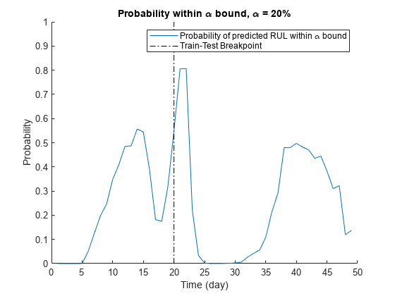
Visualize the probability of the predicted RUL within the bound.
figure
t = 1:totalDay;
hold on
plot(t, prob)
plot([breakpoint breakpoint], [0 1], 'k-.')
hold off
xlabel(['Time (' timeUnit ')'])
ylabel('Probability')
legend('Probability of predicted RUL within \alpha bound', 'Train-Test Breakpoint')
title(['Probability within \alpha bound, \alpha = ' num2str(alpha*100) '%'])
References
[1] Bechhoefer, Eric, Brandon Van Hecke, and David He. "Processing for improved spectral analysis." Annual Conference of the Prognostics and Health Management Society, New Orleans, LA, Oct. 2013.
[2] Ali, Jaouher Ben, et al. "Online automatic diagnosis of wind turbine bearings progressive degradations under real experimental conditions based on unsupervised machine learning." Applied Acoustics 132 (2018): 167-181.
[3] Saidi, Lotfi, et al. "Wind turbine high-speed shaft bearings health prognosis through a spectral Kurtosis-derived indices and SVR." Applied Acoustics 120 (2017): 1-8.
[4] Coble, Jamie Baalis. "Merging data sources to predict remaining useful life–an automated method to identify prognostic parameters." (2010).
[5] Saxena, Abhinav, et al. "Metrics for offline evaluation of prognostic performance." International Journal of Prognostics and Health Management 1.1 (2010): 4-23.