Automotive Adaptive Cruise Control Using FMCW and MFSK Technology
This example shows how to model an automotive radar in Simulink® that includes adaptive cruise control (ACC), which is an important function of an advanced driver assistance system (ADAS). The example explores scenarios with a single target and multiple targets. It shows how frequency-modulated continuous-wave (FMCW) and multiple frequency-shift keying (MFSK) waveforms can be processed to estimate the range and speed of surrounding vehicles.
Available Example Implementations
This example includes four Simulink models:
FMCW Radar Range Estimation: slexFMCWExample.slx
FMCW Radar Range and Speed Estimation of Multiple Targets: slexFMCWMultiTargetsExample.slx
MFSK Radar Range and Speed Estimation of Multiple Targets: slexMFSKMultiTargetsExample.slx
FMCW Radar Range, Speed, and Angle Estimation of Multiple Targets: slexFMCWMultiTargetsDOAExample.slx
FMCW Radar Range Estimation
The following model shows an end-to-end FMCW radar system. The system setup is similar to the MATLAB® Automotive Adaptive Cruise Control Using FMCW Technology example. The only difference between this model and the aforementioned example is that this model has an FMCW waveform sweep that is symmetric around the carrier frequency.

The figure shows the signal flow in the model. The Simulink blocks that make up the model are divided into two major sections, the Radar section and the Channel and Target section. The shaded block on the left represents the radar system. In this section, the FMCW signal is generated and transmitted. This section also contains the receiver that captures the radar echo and performs a series of operations, such as dechirping and pulse integration, to estimate the target range. The shaded block on the right models the propagation of the signal through space and its reflection from the car. The output of the system, the estimated range in meters, is shown in the display block on the left.
Radar
The radar system consists of a co-located transmitter and receiver mounted on a vehicle moving along a straight road. It contains the signal processing components needed to extract the information from the returned target echo.
FMCW- Creates an FMCW signal. The FMCW waveform is a common choice in automotive radar, because it provides a way to estimate the range using a continuous wave (CW) radar. The distance is proportional to the frequency offset between the transmitted signal and the received echo. The signal sweeps a bandwidth of 150 MHz.Transmitter- Transmits the waveform. The operating frequency of the transmitter is 77 GHz.Receiver Preamp- Receives the target echo and adds the receiver noise.Radar Platform- Simulates the radar vehicle trajectory.Signal Processing- Processes the received signal and estimates the range of the target vehicle.
Within the Radar, the target echo goes through several signal processing steps before the target range can be estimated. The signal processing subsystem consists of two high-level processing stages.
Stage 1: The first stage dechirps the received signal by multiplying it with the transmitted signal. This operation produces a beat frequency between the target echo and the transmitted signal. The target range is proportional to the beat frequency. This operation also reduces the bandwidth required to process the signal. Next, 64 sweeps are buffered to form a datacube. The datacube dimensions are fast-time versus slow-time. This datacube is then passed to a
Matrix Sumblock, where the slow-time samples are integrated to boost the signal-to-noise ratio. The data is then passed to theRange Responseblock, which performs an FFT operation to convert the beat frequency to range. Radar signal processing lends itself well to parallelization, so the radar data is then partitioned in range into 5 parts prior to further processing.Stage 2: The second stage consists of 5 parallel processing chains for the detection and estimation of the target.
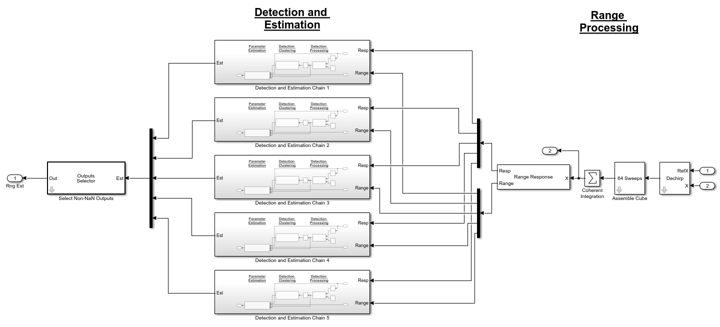
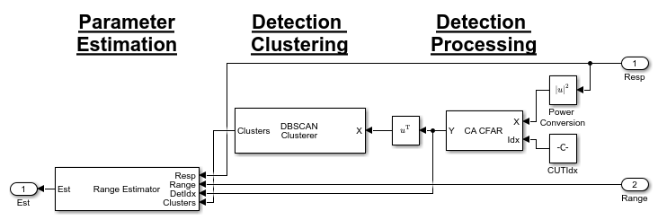
Within Stage 2, each Detection and Estimation Chain block consists of 3 processing steps.
Detection Processing: The radar data is first passed to a 1-dimensional cell-averaging (CA) constant false alarm rate (CFAR) detector that operates in the range dimension. This block identifies detections or hits.
Detection Clustering: The detections are then passed to the next step where they are aggregated into clusters using the Density-Based Spatial Clustering of Applications with Noise algorithm in the
DBSCAN Clustererblock. The clustering block clusters the detections in range using the detections identified by theCA CFARblock.Parameter Estimation: After detections and clusters are identified, the last step is the
Range Estimatorblock. This step estimates the range of the detected targets in the radar data.
Channel and Target
The Channel and Target part of the model simulates the signal propagation and reflection off the target vehicle.
Channel- Simulates the signal propagation between the radar vehicle and the target vehicle. The channel can be set as either a line-of-sight free space channel or a two-ray channel where the signal arrives at the receiver via both the direct path and the reflected path off the ground. The default choice is a free space channel.
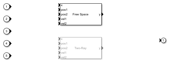
Car- Reflects the incident signal and simulates the target vehicle trajectory. The subsystem, shown below, consist of two parts: a target model to simulate the echo and a platform model to simulate the dynamics of the target vehicle.

In the Car subsystem, the target vehicle is modeled as a point target with a specified radar cross section. The radar cross section is used to measure how much power can be reflected from a target.
In this model's scenario, the radar vehicle starts at the origin, traveling at 100 km/h (27.8 m/s), while the target vehicle starts at 43 meters in front of the radar vehicle, traveling at 96 km/h (26.7 m/s). The positions and velocities of both the radar and the target vehicles are used in the propagation channel to calculate the delay, Doppler, and signal loss.
Exploring the Model
Several dialog parameters of the model are calculated by the helper function helperslexFMCWParam. To open the function from the model, click on Modify Simulation Parameters block. This function is executed once when the model is loaded. It exports to the workspace a structure whose fields are referenced by the dialogs. To modify any parameters, either change the values in the structure at the command prompt or edit the helper function and rerun it to update the parameter structure.
Results and Displays
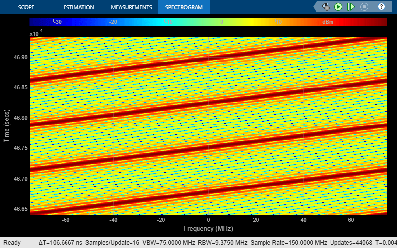
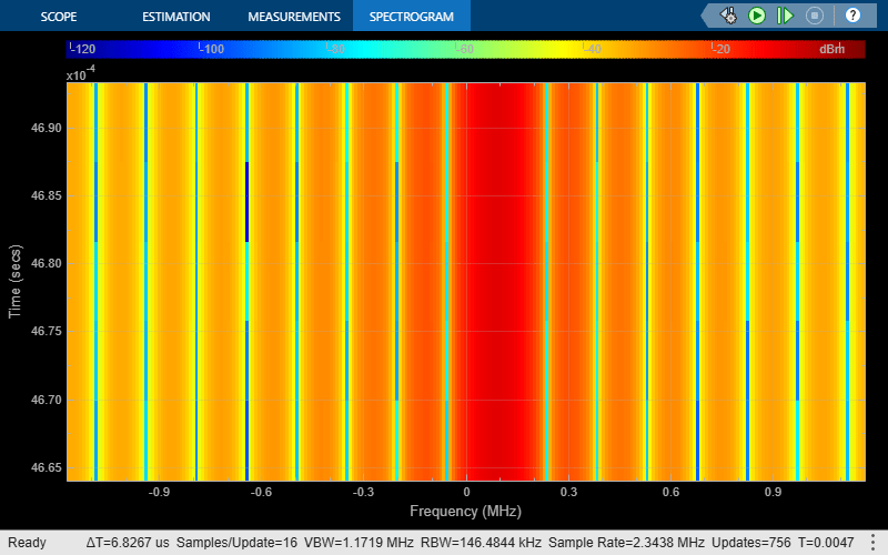
The spectrogram of the FMCW signal below shows that the signal linearly sweeps a span of 150 MHz approximately every 7 microseconds. This waveform provides a resolution of approximately 1 meter.
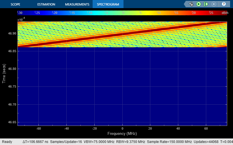
The spectrum of the dechirped signal is shown below. The figure indicates that the beat frequency introduced by the target is approximately 100 kHz. Note that after dechirp, the signal has only a single frequency component. The resulting range estimate calculated from this beat frequency, as displayed in the overall model above, is well within the 1 meter range resolution.
However, this result is obtained with the free space propagation channel. In reality, the propagation between vehicles often involves multiple paths between the transmitter and the receiver. Therefore, signals from different paths may add either constructively or destructively at the receiver. The following section sets the propagation to a two-ray channel, which is the simplest multipath channel.

Run the simulation and observe the spectrum of the dechirped signal.
Note that there is no longer a dominant beat frequency, because at this range, the signal from the direct path and the reflected path combine destructively, thereby canceling each other out. This can also be seen from the estimated range, which no longer matches the ground truth.
FMCW Radar Range and Speed Estimation of Multiple Targets
The example model below shows a similar end-to-end FMCW radar system that simulates 2 targets. This example estimates both the range and the speed of the detected targets.
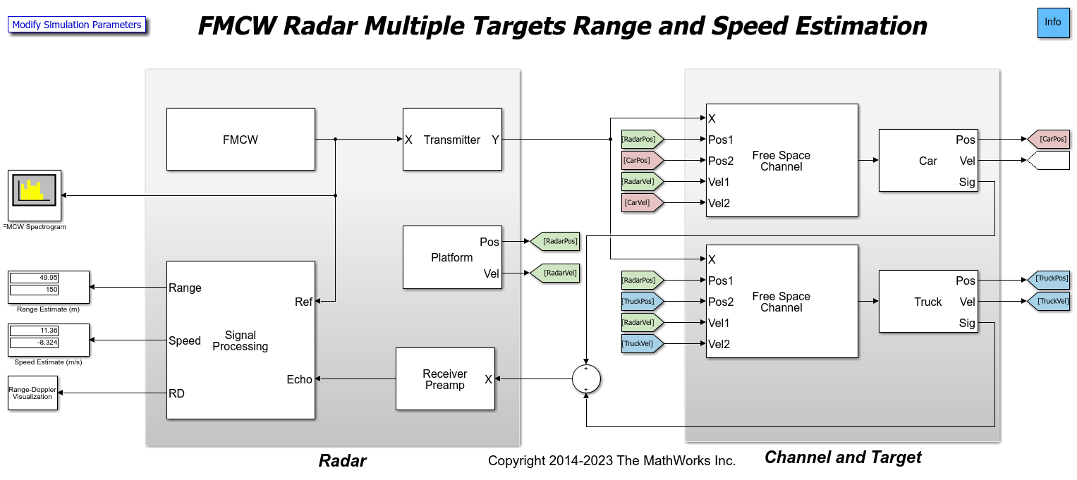
The model is essentially the same as the previous example with 4 primary differences. This model:
contains two targets,
uses range-Doppler joint processing, which occurs in the
Range-Doppler Responseblock,processes only a subset of the data in range rather than the whole datacube in multiple chains, and
performs detection using a 2-dimensional CA CFAR.
Radar
This model uses range-Doppler joint processing in the signal processing subsystem. Joint processing in the range-Doppler domain makes it possible to estimate the Doppler across multiple sweeps and then to use that information to resolve the range-Doppler coupling, resulting in better range estimates.
The signal processing subsystem is shown in detail below.
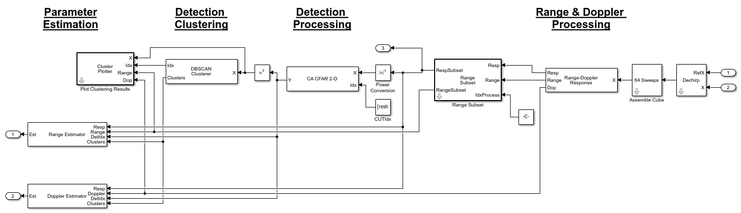
The stages that make up the signal processing subsystem are similar to the prior example. Each stage performs the following actions.
Stage 1: The first stage again performs dechirping and assembly of a datacube with 64 sweeps. The datacube is then passed to the
Range-Doppler Responseblock to compute the range-Doppler map of the input signal. The datacube is then passed to theRange Subsetblock, which obtains a subset of the datacube that will undergo further processing.Stage 2: The second stage is where the detection processing occurs. The detector in this example is the
CA CFAR 2-Dblock that operates in both the range and Doppler dimensions.Stage 3: Clustering occurs in the
DBSCAN Clustererblock using both the range and Doppler dimensions. Clustering results are then displayed by thePlot Clustersblock.Stage 4: The fourth and final stage estimates the range and speed of the targets from the range-Doppler map using the
Range EstimatorandDoppler Estimatorblocks, respectively.
As mentioned in the beginning of the example, FMCW radar uses a frequency shift to derive the range of the target. However, the motion of the target can also introduce a frequency shift due to the Doppler effect. Therefore, the beat frequency has both range and speed information coupled. Processing range and Doppler at the same time lets us remove this ambiguity. As long as the sweep is fast enough so that the target remains in the same range gate for several sweeps, the Doppler can be calculated across multiple sweeps and then be used to correct the initial range estimates.
Channel and Target
There are now two target vehicles in the scene, labeled as Car and Truck, and each vehicle has an associated propagation channel. The Car starts 50 meters in front of the radar vehicle and travels at a speed of 60 km/h (16.7 m/s). The Truck starts at 150 meters in front of the radar vehicle and travels at a speed of 130 km/h (36.1 m/s).
Exploring the Model
Several dialog parameters of the model are calculated by the helper function helperslexFMCWMultiTargetsParam. To open the function from the model, click on Modify Simulation Parameters block. This function is executed once when the model is loaded. It exports to the workspace a structure whose fields are referenced by the dialogs. To modify any parameters, either change the values in the structure at the command prompt or edit the helper function and rerun it to update the parameter structure.
Results and Displays
The FMCW signal shown below is the same as in the previous model.
The two targets can be visualized in the range-Doppler map below.
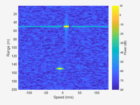
The map correctly shows two targets: one at 50 meters and one at 150 meters. Because the radar can only measure the relative speed, the expected speed values for these two vehicles are 11.1 m/s and -8.3 m/s, respectively, where the negative sign indicates that the Truck is moving away from the radar vehicle. The exact speed estimates may be difficult to infer from the range-Doppler map, but the estimated ranges and speeds are shown numerically in the display blocks in the model on the left. As can be seen, the speed estimates match the expected values well.
MFSK Radar Range and Speed Estimation of Multiple Targets
To be able to do joint range and speed estimation using the above approach, the sweep needs to be fairly fast to ensure the vehicle is approximately stationary during the sweep. This often translates to higher hardware cost. MFSK is a new waveform designed specifically for automotive radar so that it can achieve simultaneous range and speed estimation with longer sweeps.
The example below shows how to use MFSK waveform to perform the range and speed estimation. The scene setup is the same as the previous model.
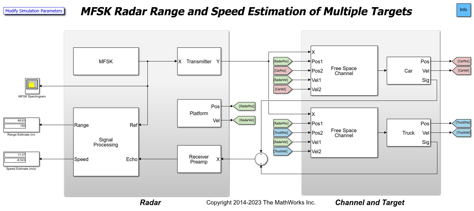
The primary differences between this model and the previous are in the waveform block and the signal processing subsystem. The MFSK waveform essentially consists of two FMCW sweeps with a fixed frequency offset. The sweep in this case happens at discrete steps. From the parameters of the MFSK waveform block, the sweep time can be computed as the product of the step time and the number of steps per sweep. In this example, the sweep time is slightly over 2 ms, which is several orders larger than the 7 microseconds for the FMCW used in the previous model. For more information on the MFSK waveform, see the Simultaneous Range and Speed Estimation Using MFSK Waveform example.
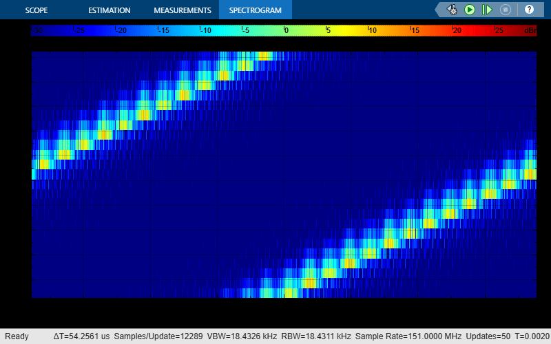
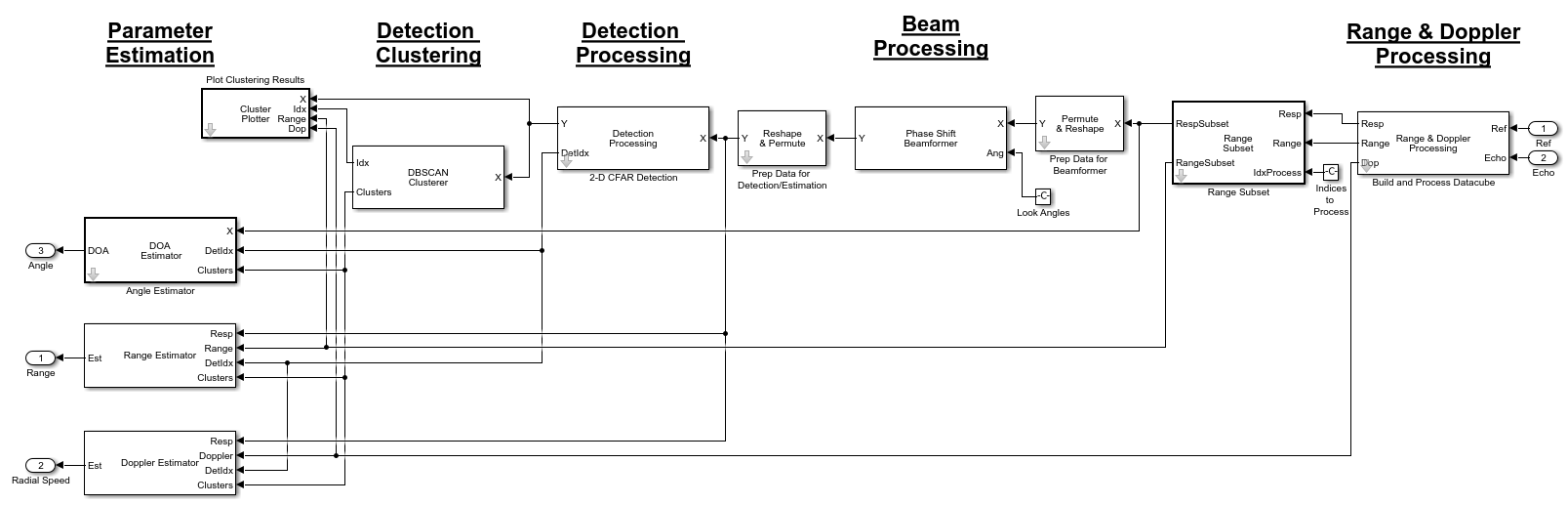
The signal processing subsystem describes how the signal gets processed for the MFSK waveform. The signal is first sampled at the end of each step and then converted to the frequency domain via an FFT. A 1-dimensional CA CFAR detector is used to identify the peaks, which correspond to targets, in the spectrum. Then the frequency at each peak location and the phase difference between the two sweeps are used to estimate the range and speed of the target vehicles.

Exploring the Model
Several dialog parameters of the model are calculated by the helper function helperslexMFSKMultiTargetsParam. To open the function from the model, click on Modify Simulation Parameters block. This function is executed once when the model is loaded. It exports to the workspace a structure whose fields are referenced by the dialogs. To modify any parameters, either change the values in the structure at the command prompt or edit the helper function and rerun it to update the parameter structure.
Results and Displays
The estimated results are shown in the model, matching the results obtained from the previous model.
FMCW Radar Range, Speed, and Angle Estimation of Multiple Targets
One can improve the angular resolution of the radar by using an array of antennas. This example shows how to resolve three target vehicles traveling in separate lanes ahead of a vehicle carrying an antenna array.

In this scenario, the radar is traveling in the center lane of a highway at 100 km/h (27.8 m/s). The first target vehicle is traveling 20 meters ahead in the same lane as the radar at 85 km/h (23.6 m/s). The second target vehicle is traveling at 125 km/h (34.7 m/s) in the right lane and is 40 meters ahead. The third target vehicle is traveling at 110 km/h (30.6 m/s) in the left lane and is 80 meters ahead. The antenna array of the radar vehicle is a 4-element uniform linear array (ULA).
The origin of the scenario coordinate system is at the radar vehicle. The ground truth range, speed, and angle of the target vehicles with respect to the radar are
                Range (m)      Speed (m/s)        Angle (deg)
  ---------------------------------------------------------------
    Car 1         20               4.2               0
    Car 2         40.05           -6.9              -2.9
    Car 3         80.03           -2.8               1.4
The signal processing subsystem now includes direction of arrival estimation in addition to the range and Doppler processing.
The processing is very similar to the previously discussed FMCW Multiple Target model. However, in this model, there are 5 stages instead of 4.
Stage 1: Similar to the previously discussed FMCW Multiple Target model, this stage performs dechirping, datacube formation, and range-Doppler processing. The datacube is then passed to the
Range Subsetblock, thereby obtaining the subset of the datacube that will undergo further processing.Stage 2: The second stage is the
Phase Shift Beamformerblock where beamforming occurs based on the specified look angles that are defined in the parameter helper function helperslexFMCWMultiTargetsDOAParam.Stage 3: The third stage is where the detection processing occurs. The detector in this example is again the
CA CFAR 2-Dblock that operates in both the range and Doppler dimensions.Stage 4: Clustering occurs in the
DBSCAN Clustererblock using the range, Doppler, and angle dimensions. Clustering results are then displayed by thePlot Clustersblock.Stage 5: The fourth and final stage estimates the range and speed of the targets from the range-Doppler map using the
Range EstimatorandDoppler Estimatorblocks, respectively. In addition, direction of arrival (DOA) estimation is performed using a custom block that features an implementation of the Phased Array System Toolbox™ Root MUSIC Estimator.
Exploring the Model
Several dialog parameters of the model are calculated by the helper function helperslexFMCWMultiTargetsDOAParam. To open the function from the model, click on Modify Simulation Parameters block. This function is executed once when the model is loaded. It exports to the workspace a structure whose fields are referenced by the dialogs. To modify any parameters, either change the values in the structure at the command prompt or edit the helper function and rerun it to update the parameter structure.
Results and Displays
The estimated results are shown in the model and match the expected values well.
Summary
The first model shows how to use an FMCW radar to estimate the range of a target vehicle. The information derived from the echo, such as the distance to the target vehicle, are necessary inputs to a complete automotive ACC system.
The example also discusses how to perform combined range-Doppler processing to derive both range and speed information of target vehicles. However, it is worth noting that when the sweep time is long, the system capability for estimating the speed is degraded, and it is possible that the joint processing can no longer provide accurate compensation for range-Doppler coupling. More discussion on this topic can be found in the MATLAB Automotive Adaptive Cruise Control Using FMCW Technology example.
The following model shows how to perform the same range and speed estimation using an MFSK waveform. This waveform can achieve the joint range and speed estimation with longer sweeps, thus reducing the hardware requirements.
The last model is an FMCW radar featuring an antenna array that performs range, speed, and angle estimation.