MTI Improvement Factor for Land-Based Radar

Open Live Script

This example discusses the moving target indication (MTI) improvement factor and investigates the effects of the following on MTI performance:

Frequency
Pulse repetition frequency (PRF)
Number of pulses
Coherent versus noncoherent processing

This example also introduces sources of error that limit MTI cancellation. Lastly, the example shows the improvement in clutter-to-noise ratio (CNR) for a land-based, MTI radar system.

MTI Improvement Factor

At a high-level, there are two types of MTI processing, coherent and noncoherent. Coherent MTI refers to the case in which the transmitter is coherent over the number of pulses used in the MTI canceler or when the coherent oscillator of the system receiver is locked to the transmitter pulse, which is also known as a coherent-on-receive system. A noncoherent MTI system uses samples of the clutter to establish a reference phase against which the target and clutter are detected.

The MTI improvement factor $I_{m}$ is defined as

$I_{m} = \frac{C_{i}}{C_{o}}$ ,

where $C_{i}$ is the clutter power into the receiver and $C_{o}$ is the clutter power after MTI processing.

Effect of Frequency

Investigate the effect of frequency on MTI performance using the mtifactor function. Use a pulse repetition frequency (PRF) of 500 Hz and analyze for 1- through 3-delay MTI cancelers for both the coherent and noncoherent cases.

% Setup parameters
m    = 2:4;                     % Number of pulses in (m-1) delay canceler
freq = linspace(1e9,10e9,1000); % Frequency (Hz)
prf  = 500;                     % Pulse repetition frequency (Hz)

% Initialize outputs
numM          = numel(m);
numFreq       = numel(freq);
ImCoherent    = zeros(numFreq,numM);
ImNoncoherent = zeros(numFreq,numM);

% Calculate MTI improvement factor versus frequency
for im = 1:numM
    % Coherent MTI 
    ImCoherent(:,im) = mtifactor(m(im),freq,prf,'IsCoherent',true);
    
    % Noncoherent MTI 
    ImNoncoherent(:,im) = mtifactor(m(im),freq,prf,'IsCoherent',false);
end

% Plot results
helperPlotLogMTI(m,freq,ImCoherent,ImNoncoherent);

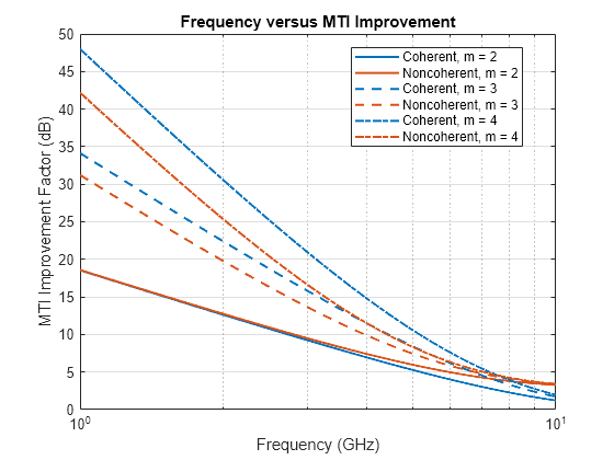
There are several takeaways from the results. First, the difference between the coherent and noncoherent results decreases with increasing frequency for the same m for the m = 3 and 4 cases. The results for the m = 2 case show that the improvement factor is very similar at lower frequencies but performance diverges at higher frequencies. Second, increasing m improves the clutter cancellation for both coherent and noncoherent MTI. Third, when the PRF is held constant, the MTI improvement factor decreases with increasing frequency. Lastly, for m = 3 and 4, the coherent performance is better than the noncoherent performance.

Effect of PRF

Next, consider the effect of PRF on the performance of the MTI filter. Calculate results for an L-band frequency at 1.5 GHz.

% Set parameters
m    = 2:4;                     % Number of pulses in (m-1) delay canceler
freq = 1.5e9;                   % Frequency (Hz)
prf  = linspace(100,1000,1000); % Pulse repetition frequency (Hz)

% Calculate MTI improvement factor versus PRF
for im = 1:numM
    ImCoherent(:,im) = mtifactor(m(im),freq,prf,'IsCoherent',true); 
    ImNoncoherent(:,im) = mtifactor(m(im),freq,prf,'IsCoherent',false); 
end

% Plot results
helperPlotMTI(m,prf,ImCoherent,ImNoncoherent,'Pulse Repetition Frequency (Hz)','PRF versus MTI Improvement');

When frequency is held constant, there are several results to note. First, the difference between the coherent and noncoherent improvement factors increase for increasing frequency for the same m for the m = 3 and 4 cases. The results for the m = 2 case show that the improvement factor is very similar over the majority of PRFs investigated. Second, the MTI performance improves with increasing PRF. Lastly, for m = 3 and 4, the coherent performance is better than the noncoherent performance.

Combined Effects of Frequency and PRF

Next, consider the combined effects of frequency and PRF on the MTI improvement factor. This will allow a system analyst to get a better sense of the entire analysis space. Perform the calculation for a coherent MTI system using a 3-delay canceler.

% Set parameters
m    = 4;                      % Number of pulses in (m-1) delay canceler
freq = linspace(1e9,10e9,100); % Frequency (Hz)
prf  = linspace(100,1000,100); % Pulse repetition frequency (Hz)

% Initialize 
numFreq          = numel(freq); 
numPRF           = numel(prf); 
ImCoherentMatrix = zeros(numPRF,numFreq); 

% Calculate coherent MTI improvement factor over a range of PRFs and
% frequencies
for ip = 1:numPRF
    ImCoherentMatrix(ip,:) = mtifactor(m,freq,prf(ip),'IsCoherent',true); 
end

% Plot results
helpPlotMTImatrix(m,freq,prf,ImCoherentMatrix);

Note that the same behaviors as previously noted are shown here:

MTI performance improves with increasing PRF
MTI performance decreases with increasing frequency

MTI Performance Limitations

MTI processing is based on a requirement of target and clutter stationarity within a receive window. When successive returns are received and subtracted from one another, clutter is canceled. Any effect, whether internal or external to the radar, that inhibits stationarity within the receive window will result in imperfect cancellation.

A wide variety of effects can decrease the performance of the MTI cancellation. Examples include but are not limited to:

Transmitter frequency instabilities
Pulse repetition interval (PRI) jitter
Pulse width jitter
Quantization noise
Uncompensated motion either in the radar platform or the clutter

The next two sections will discuss the effects of null velocity errors and clutter spectrum spread.

Null Velocity Errors

MTI performance declines when the clutter velocity is not centered on the null velocity. The effect of these null velocity errors results in a decreased MTI improvement factor since more clutter energy exists outside of the MTI filter null.

Consider the case of a radar operating in an environment with rain. Rain clutter has a non-zero average Doppler as the clutter approaches or recedes from the radar system. Unless the motion of the rain clutter is detected and compensated, the cancellation of the MTI filtering will be worse.

In this example, assume a null velocity centered at 0 Doppler. Investigate the effects on the improvement factor given clutter velocities over the range of -20 to 20 m/s for the coherent MTI processing case.

% Setup parameters
m        = 2:4;                     % Number of pulses in (m-1) delay canceler                      
clutterVels = linspace(-20,20,100); % MTI null velocity (m/s)
nullVel  = 0;                       % True clutter velocity (m/s)
freq     = 1.5e9;                   % Frequency (Hz)
prf      = 500;                     % Pulse repetition frequency (Hz)

% Initialize
numM          = numel(m);
numVels       = numel(clutterVels); 
ImCoherent    = zeros(numVels,numM); 
ImNoncoherent = nan(numVels,numM); 

% Compute MTI improvement factor 
for im = 1:numM
    for iv = 1:numVels
        ImCoherent(iv,im) = mtifactor(m(im),freq,prf,'IsCoherent',true,'ClutterVelocity',clutterVels(iv),'NullVelocity',nullVel);
    end
end

% Plot results
nullError = (clutterVels - nullVel).'; 
helperPlotMTI(m,nullError,ImCoherent,ImNoncoherent,'Null Error (m/s)','MTI Improvement with Null Velocity Errors');

The coherent MTI experiences a rapid decrease in the improvement as the null error increases. The rate at which the improvement suffers increases with increasing number of pulses in the (m-1) delay canceler. In the case where m = 4, only a slight offset of 1.1 m/s results in a loss in the improvement factor of 3 dB.

Clutter Spread

A wider clutter spread results in more clutter energy outside of an MTI filter null and thus results in less clutter cancellation. While clutter spread is due in part to the inherent motion of the clutter scatterers, other sources of clutter spread can be due to:

Phase jitter due to sampling
Phase drift, which can be due to instability in coherent local oscillators
Uncompensated radar platform motion

Consider the effect of the clutter spread on the MTI improvement factor.

% Setup parameters
m        = 2:4;                  % Number of pulses in (m-1) delay canceler
sigmav   = linspace(0.1,10,100); % Standard deviation of clutter spread (m/s)
freq     = 1.5e9;                % Frequency (Hz)
prf      = 500;                  % Pulse repetition frequency (Hz)

% Calculate MTI improvement
numSigma = numel(sigmav);
for im = 1:numM
    for is = 1:numSigma
        ImCoherent(is,im) = mtifactor(m(im),freq,prf,'IsCoherent',true,'ClutterStandardDeviation',sigmav(is));
        ImNoncoherent(is,im) = mtifactor(m(im),freq,prf,'IsCoherent',false,'ClutterStandardDeviation',sigmav(is));
    end
end

% Plot results
helperPlotMTI(m,sigmav,ImCoherent,ImNoncoherent,'Standard Deviation of Clutter Spread (m/s)','MTI Improvement versus Clutter Spread');

As can be seen from the figure, the standard deviation of the clutter spread is a great limiting factor of the MTI improvement regardless of whether the MTI is coherent or noncoherent. As the standard deviation of the clutter spread increases, the MTI improvement factor decreases significantly until the improvement falls below 5 dB for all values of m in both coherent and non-coherent cases.

Clutter Analysis for a Land-Based, MTI Radar

Consider a land-based MTI radar system. Calculate the clutter-to-noise ratio with and without MTI processing.

First, setup the radar and MTI processing parameters.

% Radar properties
freq    = 1.5e9;   % L-band frequency (Hz) 
anht    = 15;      % Height (m) 
ppow    = 100e3;   % Peak power (W)
tau     = 1.5e-6;  % Pulse width (sec)
prf     = 500;     % PRF (Hz)
Gtxrx   = 45;      % Tx/Rx gain (dB) 
Ts      = 450;     % Noise figure (dB)
Ntx     = 20;      % Number of transmitted pulses

% MTI settings 
nullVel = 0;       % Null velocity (m/s)
m       = 4;       % Number of pulses in the (m-1) delay canceler
N       = Ntx - m; % Number of coherently integrated pulses

Consider a low-relief, wooded operating environment with a clutter spread of 1 m/s and a mean clutter velocity of 0 m/s. Calculate the land surface reflectivity for the grazing angles of the defined geometry. Use the landroughness and landreflectivity functions for the physical surface properties and reflectivity calculation, respectively. For this example, use the Nathanson land reflectivity model.

% Clutter properties
sigmav     = 1;    % Standard deviation of clutter spread (m/s)
clutterVel = 0;    % Clutter velocity (m/s)
landType   = 'Woods'; 

% Get the surface standard deviation of height (m), surface slope (deg),
% and vegetation type
[surfht,beta0,vegType] = landroughness(landType); 

% Calculate maximum range for simulation
Rua = time2range(1/prf); % Maximum unambiguous range (m)
Rhoriz = horizonrange(anht,'SurfaceHeight',surfht); % Horizon range (m)
RhorizKm = Rhoriz.*1e-3; % Horizon range (km)
Rmax = min(Rua,Rhoriz); % Maximum range (m)

% Generate vector of ranges for simulation
Rm  = linspace(100,Rmax,1000); % Range (m)
Rkm = Rm*1e-3;                 % Range (km) 

% Calculate land clutter reflectivity using Nathanson's land reflectivity
% model
grazAng = grazingang(anht,Rm,'TargetHeight',surfht); 
nrcs = landreflectivity(landType,grazAng,freq,'Model','Nathanson'); 
nrcsdB = pow2db(nrcs);

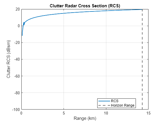
Next, calculate and plot the radar cross section (RCS) of the clutter using the clutterSurfaceRCS function. The vertical line denotes the horizon.

% Calculate azimuth and elevation beamwidth
azbw = sqrt(32400/db2pow(Gtxrx));
elbw = azbw;

% Calculate clutter RCS
rcs = clutterSurfaceRCS(nrcs,Rm,azbw,elbw,grazAng(:),tau); 

% Plot clutter RCS including horizon line
rcsdB = pow2db(rcs); % Convert to decibels for plotting
hAxes = helperPlot(Rkm,rcsdB,'RCS','Range (km)','Clutter RCS (dBsm)','Clutter Radar Cross Section (RCS)');
helperAddHorizLine(hAxes,RhorizKm);

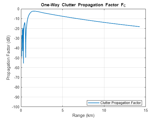
Since the propagation path deviates from free space, include the clutter propagation factor and atmospheric losses in the calculation.

The default permittivity calculation underlying the radarpropfactor function is a sea water model. In order to more accurately simulate the propagation path over land, calculate the permittivity for the vegetation using the earthSurfacePermittivity function.

% Calculate land surface permittivity for vegetation
temp = 20; % Ambient temperature (C)
wc = 0.5;  % Gravimetric water contnt
epsc = earthSurfacePermittivity('vegetation',freq,temp,wc);

Calculate the clutter propagation factor using the radarpropfactor function. Include the vegetation type in the calculation. At higher frequencies, the presence of vegetation can cause additional losses.

% Calculate clutter propagation factor 
Fc = radarpropfactor(Rm,freq,anht,surfht, ... 
    'SurfaceHeightStandardDeviation',surfht, ...
    'SurfaceSlope',beta0, ...
    'VegetationType',vegType, ...
    'SurfaceRelativePermittivity',epsc, ...
    'ElevationBeamwidth',elbw);
helperPlot(Rkm,Fc,'Clutter Propagation Factor','Range (km)', ...
    'Propagation Factor (dB)', ...
    'One-Way Clutter Propagation Factor F_C');

Next, calculate the atmospheric losses in this simulation. Assume the default standard atmosphere. Perform the calculation using the tropopl function.

% Calculate the atmospheric loss due to water and oxygen attenuation
elAng = height2el(surfht,anht,Rm); % Elevation angle (deg) 
numEl = numel(elAng);
Latmos = zeros(numEl,1);
Llens = zeros(numEl,1);
for ie = 1:numEl
    Latmos(ie,:) = tropopl(Rm(ie),freq,anht,elAng(ie));
end
hAxes = helperPlot(Rkm,Latmos,'Atmospheric Loss','Range (km)','Loss (dB)','One-Way Atmospheric Losses');
ylim(hAxes,[0 0.1]);

Calculate the CNR using the radareqsnr function and plot results with and without MTI. Again, note the drop in CNR as the simulation range approaches the radar horizon.

% Calculate CNR
lambda = freq2wavelen(freq); 
cnr = radareqsnr(lambda,Rm(:),ppow,tau, ... 
        'gain',Gtxrx,'rcs',rcs,'Ts',Ts, ...
        'PropagationFactor',Fc, ...
        'AtmosphericLoss',Latmos);
coherentGain = pow2db(N);
cnr = cnr + coherentGain; 
hAxes = helperPlot(Rkm,cnr,'CNR','Range (km)','CNR (dB)','CNR Clutter-to-Noise Ratio');
helperAddHorizLine(hAxes,RhorizKm);

% Calculate CNR with MTI
Im = mtifactor(m,freq,prf,'IsCoherent',true,...
    'ClutterVelocity',clutterVel, ...
    'ClutterStandardDeviation',sigmav, ...
    'NullVelocity',nullVel)

Im = 55.3986

cnrMTI = cnr - Im; 
helperAddPlot(Rkm,cnrMTI,'CNR + MTI',hAxes);

Lastly, calculate the MTI improvement factor assuming a null error exists due to the true clutter velocity being 3 m/s while the null velocity remains centered at 0 m/s.

% Calculate CNR with null velocity error
trueClutterVel = 3;                   % Clutter velocity (m/s) 
nullError = trueClutterVel - nullVel; % Null error (m/s)
ImNullError = mtifactor(m,freq,prf,'IsCoherent',true,...
    'ClutterVelocity',trueClutterVel, ...
    'ClutterStandardDeviation',sigmav, ...
    'NullVelocity',nullVel)

ImNullError = 33.6499

cnrMTINullError = cnr - ImNullError;
helperAddPlot(Rkm,cnrMTINullError, ...
    sprintf('CNR + MTI with %.1f (m/s) Null Error',nullError), ...
    hAxes);

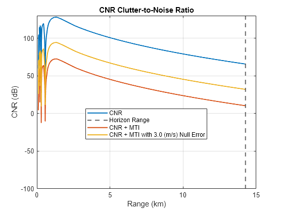
ImLoss = Im - ImNullError

ImLoss = 21.7488

Note the dramatic decrease in the CNR due to the MTI processing. When the null velocity is set to the clutter velocity, the improvement is 55 dB. When there is an uncompensated motion, the cancellation decreases to 34 dB. This is a loss of about 22 dB of cancellation. This shows the need to properly compensate for motion or to steer the null to the appropriate velocity.

Summary

This example discusses the MTI improvement factor and investigates a multitude of effects on MTI performance. Using the mtifactor function, we see that MTI performance:

Improves with increasing PRF
Decreases with increasing frequency
Improves with increasing the number of pulses in the (m - 1)-delay canceler

Additionally, we see that the performance of coherent MTI is generally better than noncoherent MTI.

Lastly, we investigate limitations of MTI performance within the context of a land-based MTI radar system, showing the need to properly compensate for unexpected clutter velocities.

References

Barton, David Knox. Radar Equations for Modern Radar. Artech House Radar Series. Boston, Mass: Artech House, 2013.
Richards, M. A., Jim Scheer, William A. Holm, and William L. Melvin, eds. Principles of Modern Radar. Raleigh, NC: SciTech Pub, 2010.

function helperPlotLogMTI(m,freq,ImCoherent,ImNonCoherent)
% Used for the MTI plots that have a logarithmic x axis

hFig = figure;
hAxes = axes(hFig);
lineStyles = {'-','--','-.'};
numM = numel(m);
for im = 1:numM
    semilogx(hAxes,freq.*1e-9,ImCoherent(:,im),'LineWidth',1.5, ...
        'LineStyle',lineStyles{im}, 'Color',[0 0.4470 0.7410], ...
        'DisplayName',sprintf('Coherent, m = %d',m(im)))
    hold(hAxes,'on')
    semilogx(hAxes,freq.*1e-9,ImNonCoherent(:,im),'LineWidth',1.5, ...
        'LineStyle',lineStyles{im}, 'Color',[0.8500 0.3250 0.0980], ...
        'DisplayName',sprintf('Noncoherent, m = %d',m(im)))
end
grid(hAxes,'on');
xlabel(hAxes,'Frequency (GHz)')
ylabel(hAxes,'MTI Improvement Factor (dB)')
title('Frequency versus MTI Improvement')
legend(hAxes,'Location','Best')
end

function helperPlotMTI(m,x,ImCoherent,ImNonCoherent,xLabelStr,titleName)
% Used for the MTI plots that have an x-axis in linear units

hFig = figure;
hAxes = axes(hFig);
lineStyles = {'-','--','-.'};
numM = numel(m);
for im = 1:numM
    plot(hAxes,x,ImCoherent(:,im),'LineWidth',1.5, ...
        'LineStyle',lineStyles{im}, 'Color',[0 0.4470 0.7410], ...
        'DisplayName',sprintf('Coherent, m = %d',m(im)))
    hold(hAxes,'on')
    if any(~isnan(ImNonCoherent)) % Don't plot if NaN
        plot(hAxes,x,ImNonCoherent(:,im),'LineWidth',1.5, ...
            'LineStyle',lineStyles{im}, 'Color',[0.8500 0.3250 0.0980], ...
            'DisplayName',sprintf('Noncoherent, m = %d',m(im)))
    end
end
grid(hAxes,'on');
xlabel(hAxes,xLabelStr)
ylabel(hAxes,'MTI Improvement Factor (dB)')
title(titleName)
legend(hAxes,'Location','Best')
end

function helpPlotMTImatrix(m,freq,prf,ImMat)
% Creates image of MTI improvement factor with Frequency on the x-axis and
% PRF on the y-axis

hFig = figure;
hAxes = axes(hFig); 
hP = pcolor(hAxes,freq.*1e-9,prf,ImMat);
hP.EdgeColor = 'none'; 
xlabel(hAxes,'Frequency (GHz)')
ylabel(hAxes,'PRF (Hz)')
title(sprintf('Coherent MTI Improvement, m = %d',m))
hC = colorbar;
hC.Label.String = '(dB)'; 
end

function varargout = helperPlot(x,y,displayName,xlabelStr,ylabelStr,titleName)
% Used for CNR analysis 

% Create new figure 
hFig = figure;
hAxes = axes(hFig);

% Plot
plot(hAxes,x,y,'LineWidth',1.5,'DisplayName',displayName);
grid(hAxes,'on');
hold(hAxes,'on');
xlabel(hAxes,xlabelStr)
ylabel(hAxes,ylabelStr);
title(hAxes,titleName);
ylims = get(hAxes,'Ylim'); 
set(hAxes,'Ylim',[-100 ylims(2)]); 

% Add legend
legend(hAxes,'Location','Best')

% Output axes
if nargout ~= 0 
    varargout{1} = hAxes;
end
end

function helperAddPlot(x,y,displayName,hAxes)
% Add additional CNR plots

plot(hAxes,x,y,'LineWidth',1.5,'DisplayName',displayName);
end

function helperAddHorizLine(hAxes,val)
% Add vertical line indicating horizon range

xline(hAxes,val,'--','DisplayName','Horizon Range','LineWidth',1.5);
end