Robust Loop Shaping of Nanopositioning Control System
This example shows how to use the Glover-McFarlane technique to obtain loop-shaping compensators with good stability margins. The example applies the technique to a nanopositioning stage. These devices can achieve very high precision positioning which is important in applications such as atomic force microscopes (AFMs). For more details on this application, see [1].
Nanopositioning System
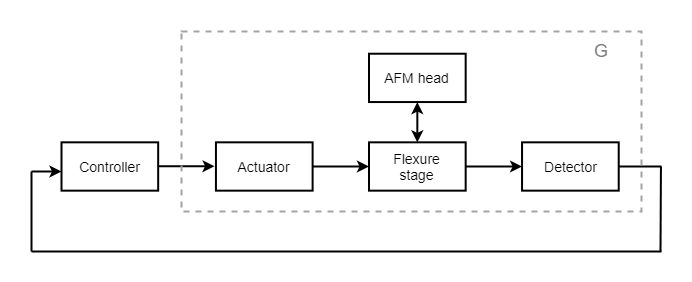
The following illustration shows a feedback diagram of a nanopositioning device. The system consists of piezo-electric actuation, a flexure stage, and a detection system. The flexure stage interacts with the head of the AFM.
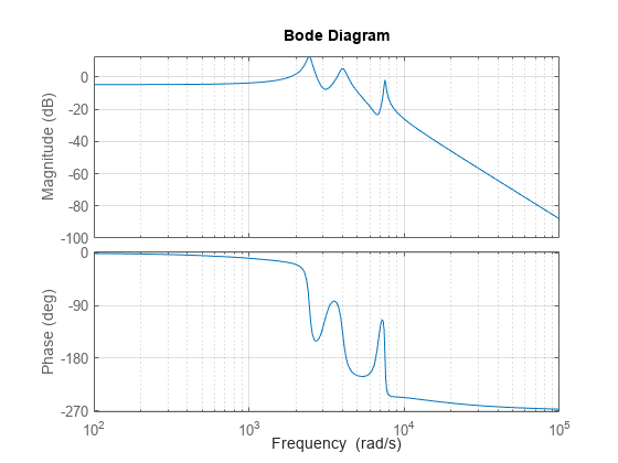
Load the plant model for the nanopositioning stage. This model is a seventh-order state-space model fitted to frequency response data obtained from the device.
load npfit A B C D
G = ss(A,B,C,D);
bode(G)
grid
Typical design requirements for the control law include high bandwidth, high resolution, and good robustness. For this example, use:
Bandwidth of approximately 50 Hz
Roll-off of -40 dB/decade past 250 Hz
Gain margin in excess of 1.5 (3.5 dB) and phase margin in excess of 60 degrees
Additionally, when the nanopositioning stage is used for scanning, the reference signal is triangular, and it is important that the stage tracks this signal with minimal error in the midsection of the triangular wave. One way of enforcing this is to add the following design requirement:
A double integrator in the control loop
PI Design
First try a PI design. To accommodate the double integrator requirement, multiply the plant by . Set the desired bandwidth to 50 Hz. Use pidtune to automatically tune the PI controller.
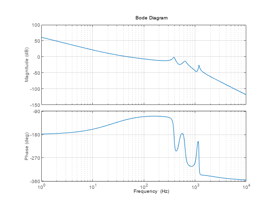
Integ = tf(1,[1 0]);
bw = 50*2*pi;  % 50 Hz in rad/s
PI = pidtune(G*Integ,'pi',50*2*pi);
C = PI*Integ;

bp = bodeplot(G*C);
bp.FrequencyUnit = 'Hz';
bp.XLimits = [1e0 1e4];
grid on
This compensator meets the bandwidth requirement and almost meets the roll-off requirement. Use allmargin to calculate the stability margins.
allmargin(G*C)
ans = struct with fields:
     GainMargin: [1.1531 13.7832 7.4195]
    GMFrequency: [2.4405e+03 3.3423e+03 3.7099e+03]
    PhaseMargin: 60.0024
    PMFrequency: 314.1959
    DelayMargin: 0.0033
    DMFrequency: 314.1959
         Stable: 1
The phase margin is satisfactory, but the smallest gain margin is only 1.15, far below the target of 1.5. You could try adding a lowpass filter to roll off faster beyond the gain crossover frequency, but this would most likely reduce the phase margin.
Glover-McFarlane Loop Shaping
The Glover-McFarlane technique provides an easy way to tweak the candidate compensator C to improve its stability margins. This technique seeks to maximize robustness (as measured by ncfmargin) while roughly preserving the loop shape of G*C. Use ncfsyn to apply this technique to this application. Note that ncfsyn assumes positive feedback so you need to flip the sign of the plant G.
[K,~,gam] = ncfsyn(-G,C);
Check the stability margins with the refined compensator K.
[Gm,Pm] = margin(G*K)
Gm =
3.7267
Pm =
70.7109
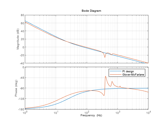
The ncfsyn compensator increases the gain margin to 3.7 and the phase margin to 70 degrees. Compare the loop shape for this compensator with the loop shape for the PI design.
bp = bodeplot(G*C,G*K);
bp.FrequencyUnit = 'Hz';
bp.XLimits = [1e0 1e4];
grid on
legend('PI design','Glover-McFarlane');
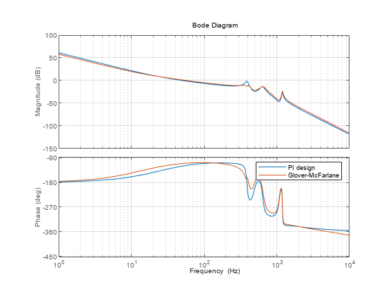
The Glover-McFarlane compensator attenuates the first resonance responsible for the weak gain margin while boosting the lead effect to preserve and even improve the phase margin. This refined design meets all requirements. Compare the two compensators.
bodeplot(C,K);
grid on
legend('PI design','Glover-McFarlane');
The refined compensator has roughly the same gain profile. ncfsyn automatically added zeros in the right places to accommodate the plant resonances.
Compensator Simplification
The ncfsyn algorithm produces a compensator of relatively high order compared to the original second-order design.
order(K)
ans =
11
You can use reducespec to reduce this down to something close to the original order. For example, try order 4.
ord = 4;
R = reducespec(K,"ncf")
R =
NCFBalancedTruncation with properties:
Sigma: []
Energy: []
Error: []
LNCF: []
TL: []
TR: []
Lr: []
Lo: []
Options: []
Kr = getrom(R,Order=ord)
Kr =

  A =
           x1      x2      x3      x4
   x1  -70.94  -355.8   520.3  -201.7
   x2   118.5    2731   -5584    1179
   x3   254.3    2773   -3365   814.4
   x4   13.47   9.803  -148.4    66.5

  B =
           u1
   x1  -60.95
   x2   18.77
   x3   29.32
   x4   1.174

  C =
           x1      x2      x3      x4
   y1  -11.97   6.355  -4.543  -75.51

  D =
       u1
   y1   0

Continuous-time state-space model.
Model Properties
[Gm,Pm] = margin(G*Kr)
Gm =
3.8139
Pm =
70.6770
bp = bodeplot(G*K,G*Kr);
bp.FrequencyUnit = 'Hz';
bp.XLimits = [1e0 1e4];
grid
legend('11th order','4th order');

The reduced-order compensator Kr has very similar loop shape and stability margins and is a reasonable candidate for implementation.
References
Salapaka, S., A. Sebastian, J. P. Cleveland, and M. V. Salapaka. “High Bandwidth Nano-Positioner: A Robust Control Approach.” Review of Scientific Instruments 73, no. 9 (September 2002): 3232–41.
See Also
ncfsyn | ncfmargin | reducespec