Eye Measurement and Reporting
The standard of performance for a high-speed serial link is bit-error-ratio (BER). BER is estimated based on a number of factors, one of which is the inner eye contour of an eye diagram. Simulation results, both statistical and time domain, contain eye width and height measurements, along with calculated margin to a target BER.
Note
The methods and reporting of these metrics pertain to Parallel Link Designer only when simulating in STAT mode.
The inner contour of the eye diagram at the Target BER is used to estimate the channel BER. Understanding the derivation of eye height, width and voltage margin as reported in statistical and time domain simulations provides insight to the BER estimate. For compliance to standards, inner and outer eye masks can be applied to simulation results and the available margin is reported. Knowing how the margin is calculated and reported is beneficial to debugging potential problems within a design.
Parameters Used in Eye Measurement
Eye metrics such as height, width and margin along with the BER for the channel are determined based on three metrics; the eye contours, the clock PDF and the sensitivity of the receiver.
Eye Contours
Eye contours are plots of the amplitude associated with fixed probabilities as a function of sampling time. They indicate the shape of the inner and outer boundaries of the eye diagram for each of a number of different probabilities. The eye contours for a given simulation are based on the Target BER.
To set the target BER, open the Simulation Parameters dialog box by selecting Setup > Simulation Parameters from the Serial Link Designer or Parallel Link Designer app.
The default value is 1e-12, but you can set this based on the BER
requirement of the channel design. Target BER defines the contours that is generated and
reported after rolling up the simulation results.
Four eye contours are generated after the simulation, for the Target BER, Target BER
+ 1e3, Target BER + 1e6 and Target BER +
1e9. For example, if the Target BER is set at
1e-12, the contours are displayed at: 1e-12,
1e-9, 1e-6 and 1e-3. Regardless
of the Target BER setting, a 0 contour is also generated which
represents the BER = 0 point.
Clock PDF
The clock PDF is the probability density function (PDF) of the phase difference between the clock at the receiver decision point and an ideal transmitter symbol clock. It is represented as a Gaussian probability density function.
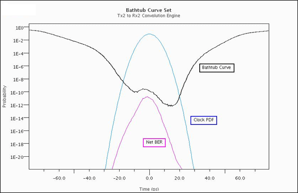
You can determine the net BER from the interaction between the bathtub curves and the clock pdf. The bathtub curve is the probability of error as a function of the time that the data is actually sampled. The net BER is the probability of an error occurring at a given sampling time given the probability of sampling at that time. This curve is the area under the product of the bathtub curve and the clock PDF.
Receiver Sensitivity
Sensitivity is a keyword that is part of the IBIS-AMI specification for receiver
models. It is defined as the minimum latch overdrive voltage at the data decision point of
the receiver after equalization. For example if sensitivity is defined as 25mV, the latch
would require +/- 25mV for switching. The default sensitivity used in the Serial Link
Designer and Parallel Link Designer is 0.
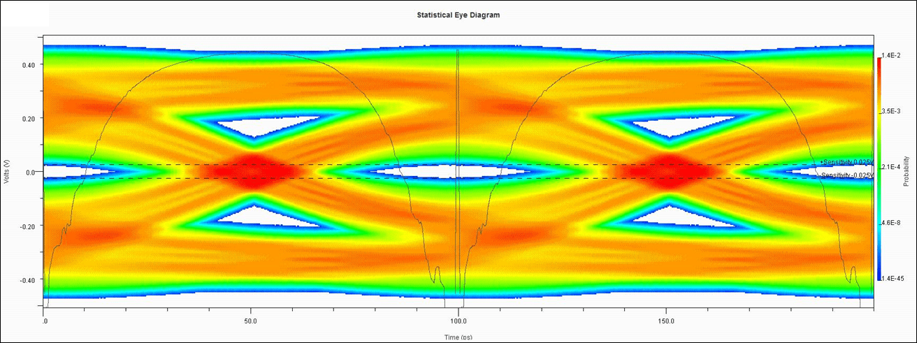
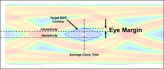
A statistical eye diagram with the bathtub curve set and the receiver sensitivity marked +/- 25mV (dashed lines) is shown:
Calculating Eye Metrics
To calculate the eye metrics, you need to first find the center eye. For even n in a PAMn modulation scheme, the center eye is considered as the eye at the zero voltage. For odd n, the center eye is considered as the first eye below the eye at the zero voltage.
The time center of the 1e-3 contour of the center eye is referred to
as Tmid time. After finding the Tmid time,
Tmid eye height and eye width are reported for the center eye using the
target BER contour. For CEI 56G PAM4 specifications, the target BER is
1e-6. The eye contour probability is measured using the cumulative
distribution function (CDF).
The tentative Vmid location of each eye is determined by searching up
at Tmid for a maximum histogram density, then continuing to search up for
a minimum eye density. This is repeated for each eye.
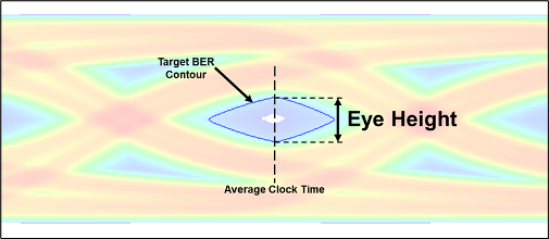
The eye height for each eye is determined by the target CDF voltage above and below the
tentative Vmid position of eye. The Vmid position of
each eye is half way between these two voltages.
The eye width of each eye is determined by the target CDF contour to the left and right
of the Tmid position and the Vmid position of each
eye.
Note
These eye widths and eye heights are measured in accordance with the CEI 56G PAM4 specifications. They do not necessarily represent the maximum eye width or eye height of each eye or the time location of the eye that is actually sampled by the hardware.
Eye Reporting
Signal Integrity Viewer reports the results of statistical simulation.
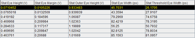
These results include statistical eye height, eye width, eye margin, outer eye height, and threshold eye width. These results are all determined from the Target BER contour and the receiver sensitivity.
| Parameter | Description | Eye Diagram Representation |
|---|---|---|
| Stat Eye Height(V) | The height of the target bit error rate contour at the average clock time. |
|
| Stat Eye Width(ps) | The width of the eye measured at the 0V crossing. |
|
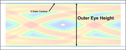
| Stat Eye Outer Height (V) | The maximum voltage measured on the outer eye. This is the maximum voltage measured on the zero outer contour. |
|
| Stat Threshold Eye Width (ps) | The eye width measured at the intersection of the inner eye and the receiver sensitivity. | |
| Stat Eye Margin (V) | Voltage measured from the sensitivity threshold to the target BER contour at the average clock time. |
|
| Stat Clock PDF Mean | The mean of the recovered clock. | |
| Stat Clock PDF Sigma | The standard deviation of the recovered clock. | |
| Stat BER | The average bit error as predicted through statistical analysis. | |
| Stat BER Floor | The minimum bit error rate at any point on the bathtub curve derived from statistical analysis. |

Eye height and eye width are reported for all contours generated in the simulation based on the Target BER.

For example, if the target BER is 1e-12, statistical eye heights and
widths for 1e-3, 1e-6, 1e-9 and
1e-12 BER are reported.
Note
When comparing the reported results to measurements made manually in Signal Integrity Viewer, an error is introduced from the samples per bit selection. To determine the amount of error when making a manual measurement, divide the UI (unit interval) of a bit by the number of samples per bit (UI/SPB). Using a higher number of samples per bit results in a smaller error.
Calculating Eye Margin from Simulation Results to Eye Mask
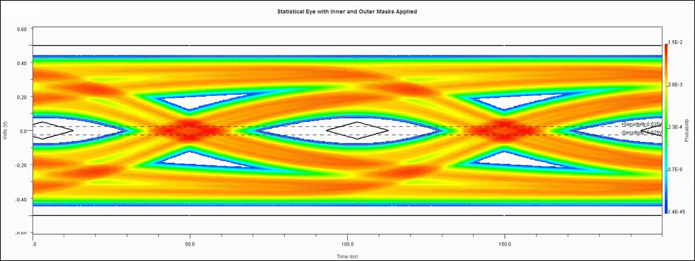
When an eye mask is defined and applied to a sheet being simulated, the margin between the mask and the Target BER contour are reported. An eye mask can be defined as either an inner mask, outer mask or both. A statistical eye diagram with inner and outer masks applied is shown:
If both inner and outer masks are defined, the smallest margin at any point of the two is reported. The worst eye height margin and worst eye width margin at any point for a given eye mask. Only one result is reported so it is important know which masks are being applied to best identify violations.
You can define and use two types of eye masks: static and skew eye masks. A static eye mask is centered at the 0.5UI point of the bit time. The margin to the mask can then be determined based on its static position. The skew eye mask is positioned by the simulator after simulation to maximize eye margin and place the mask at its optimal point in the eye
To obtain the mask margin numbers using a skew eye mask:
Slice UI into discrete time slices (for example, 256 slices per UI).
Place mask edge at zero UI and obtain margins for all time slices that cross mask (margins are positive and negative).
Increment mask to next time slice and recapture margins for all slices that cross mask.
Continue this process until right side of mask hits
1UI.
Taking all of this data, obtain the best position for the mask that maximizes the worst case margin (looking for most positive result) across all time slices. Then report the worst case margin. The determination of mask margins is shown as:
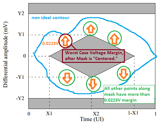
The worst case margin is shown to be between a perturbation of the eye contour and the mask. In this case no outer mask is assumed.
If both an outer mask and inner mask are applied in a simulation and a violation is reported, you need to determine where the violation comes from. A violation to the outer eye mask when both inner and outer eye masks applied is shown:
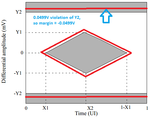
After simulation, the results for eye mask margin is reported:
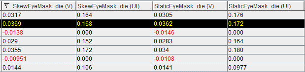
In this case both skew and static masks are applied. Eye height and width margins are reported in the individual columns. Comparing static and skew mask margins in the table below show slightly more margin when applying the skew mask. The red entries represent violations to either the upper or lower mask. To identify the violation the Target BER contour and the mask can be plotted.