Modal Analysis of a Simulated System and a Wind Turbine Blade
This example shows how to estimate frequency-response functions (FRFs) and modal parameters from experimental data. The first section describes a simulated experiment that excites a three-degree-of-freedom (3DOF) system with a sequence of hammer impacts and records the resulting displacement. Frequency-response functions, natural frequencies, damping ratios, and mode shape vectors are estimated for three modes of the structure. The second section estimates mode shape vectors from frequency-response function estimates from a wind turbine blade experiment. The turbine blade measurement configuration and resulting mode shapes are visualized. This example requires System Identification Toolbox (TM).
Natural Frequency and Damping for a Simulated Beam
Single-Input/Single-Output Hammer Excitation
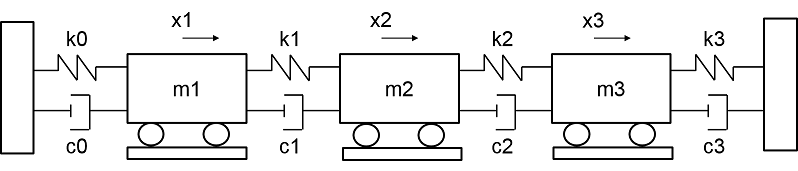
A series of hammer strikes excite a 3DOF system, and sensors record the resulting displacements. The system is proportionally damped, such that the damping matrix is a linear combination of the mass and stiffness matrices.
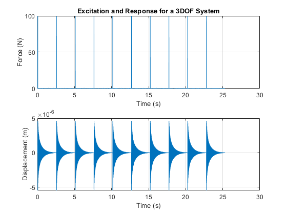
Import the data for two sets of measurements, including excitation signals, response signals, time signals, and ground truth frequency-response functions. The first set of response signals, Y1, measures the displacement of the first mass, and the second, Y2, measures the second mass. Each excitation signal consists of ten concatenated hammer impacts, and each response signal contains the corresponding displacement. The duration for each impact signal is 2.53 seconds. Additive noise is present in the excitation and response signals. Visualize the first excitation and response channel of the first measurement.
[t,fs,X1,X2,Y1,Y2,f0,H0] = helperImportModalData();
X0 = X1(:,1);
Y0 = Y1(:,1);
helperPlotModalAnalysisExample([t' X0 Y0]);
Compute and plot the FRF for the first excitation and response channels in terms of dynamic flexibility, which is a measure of displacement over force [1]. By default, the FRF is computed by averaging spectra of windowed segments. Since each hammer excitation decays substantially before the next excitation, a rectangular window can be used. Specify the sensor as displacement.
winLen = 2.5275*fs; % window length in samples
modalfrf(X0,Y0,fs,winLen,'Sensor','dis')
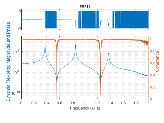
The FRF, estimated using the default 'H1' estimator, contains three prominent peaks in the measured frequency band, corresponding to three flexible modes of vibration. The coherence is close to one near these peaks, and low in anti-resonance regions, where the signal-to-noise ratio of the response measurement is low. Coherence near to one indicates a high quality estimate. The 'H1' estimate is optimal where noise exists only at the output measurement, whereas the 'H2' estimator is optimal when there is additive noise only on the input [2]. Compute the 'H1' and 'H2' estimates for this FRF.
[FRF1,f1] = modalfrf(X0,Y0,fs,winLen,'Sensor','dis');  % Calculate FRF (H1)
[FRF2,f2] = modalfrf(X0,Y0,fs,winLen,'Sensor','dis','Estimator','H2');
When there is significant measurement noise or the excitation is poor, parametric methods can offer additional options for accurately extracting the FRF from the data. The 'subspace' method first fits a state-space model to the data [3] and then computes its frequency-response function. The order of the state-space model (equal to the number of poles) and presence or lack of feedthrough can be specified to configure the state-space estimation.
[FRF3,f3] = modalfrf(X0,Y0,fs,winLen,'Sensor','dis','Estimator','subspace','Feedthrough',true);
Here FRF3 is estimated by fitting a state-space model containing a feedthrough term and of the optimal order in the range 1:10. Compare the estimated FRFs using 'H1', 'H2' and 'subspace' methods to the theoretical FRF.
helperPlotModalAnalysisExample(f1,FRF1,f2,FRF2,f3,FRF3,f0,H0);
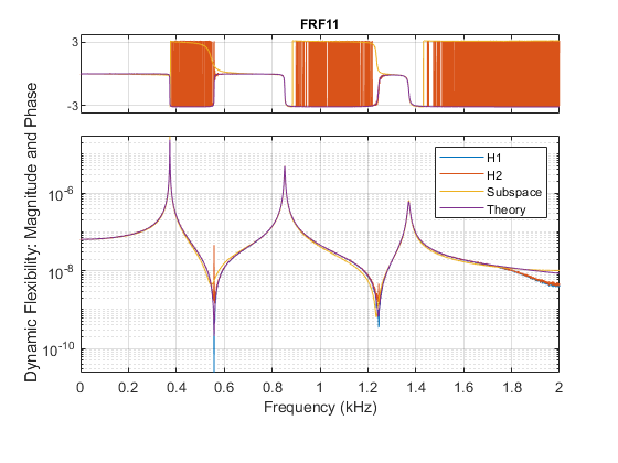
The estimators perform comparably near response peaks, while the 'H2' estimator overestimates the response at the antiresonances. The coherence is not affected by the choice of the estimator.
Next, estimate the natural frequency of each mode using the peak-picking algorithm. The peak-picking algorithm is a simple and fast procedure for identifying peaks in the FRF. It is a local method, since each estimate is generated from a single frequency-response function. It is also a single-degree-of-freedom (SDOF) method, since the peak for each mode is considered independently. As a result, a set of modal parameters is generated for each FRF. Based on the previous plot, specify a frequency range from 200 to 1600 Hz, which contains the three peaks.
fn = modalfit(FRF1,f1,fs,3,'FitMethod','PP','FreqRange',[200 1600])
fn =

   1.0e+03 *

    0.3727
    0.8525
    1.3707
The natural frequencies are approximately 373, 853, and 1371 Hz. Plot a reconstructed FRF and compare it to the measured data using modalfit. The FRF is reconstructed using the modal parameters estimated from the frequency-response function matrix, FRF1. Call modalfit again with no output arguments to produce a plot containing the reconstructed FRF.
modalfit(FRF1,f1,fs,3,'FitMethod','PP','FreqRange',[200 1600])
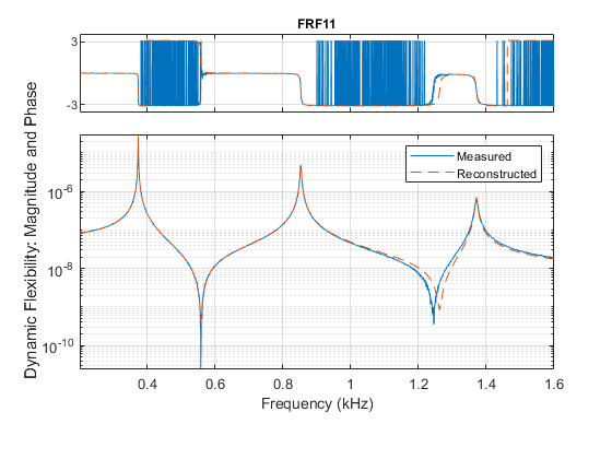
The reconstructed FRF agrees with the measured FRF of the first excitation and response channels. In the next section, two additional excitation locations are considered.
Roving Hammer Excitation
Compute and plot the FRFs for the responses of all three sensors using the default 'H1' estimator. Specify the measurement type as 'rovinginput' since we have a roving hammer excitation.
modalfrf(X1,Y1,fs,winLen,'Sensor','dis','Measurement','rovinginput')
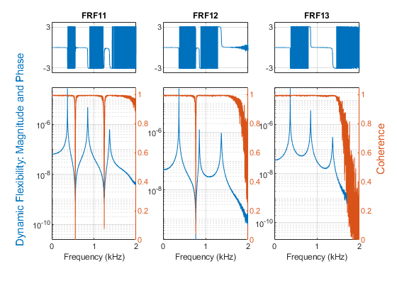
In the previous section, a single set of modal parameters was computed from a single FRF. Now, estimate modal parameters using the least-squares complex exponential (LSCE) algorithm. The LSCE and LSRF algorithms generate a single set of modal parameters by analyzing multiple response signals simultaneously. These are global, multiple-degree-of-freedom (MDOF) methods, since the parameters for all modes are estimated simultaneously from multiple frequency-response functions.
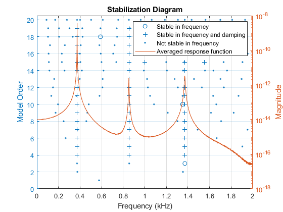
The LSCE algorithm generates computational modes, which are not physically present in the structure. Use a stabilization diagram to identify physical modes by examining the stability of poles as the number of modes increases. The natural frequencies and damping ratios of physical modes tend to remain in the same place, or are 'stable'. Create a stabilization diagram and output the natural frequencies of those poles which are stable in frequency.
[FRF,f] = modalfrf(X1,Y1,fs,winLen,'Sensor','dis','Measurement','rovinginput');
fn = modalsd(FRF,f,fs,'MaxModes',20, 'FitMethod', 'lsce'); % Identify physical modes
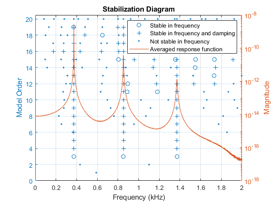
By default, poles are classified as stable in frequency if the natural frequency for the poles changes by less than one percent. Poles which are stable in frequency are further classified as stable in damping for a smaller than five percent change in damping ratio. Both criteria can be adjusted to different values. Based on the location of the stable poles, choose natural frequencies of 373, 852.5, and 1371 Hz. These frequencies are contained in the output fn of modalsd, along with natural frequencies of other frequency-stable poles. A higher model order than the number of modes physically present is generally needed to produce good modal parameters estimates using the LSCE algorithm. In this case, a model order of four modes indicates three stable poles. The frequencies of interest occur in the first three columns in the 4th row of fn.
physFreq = fn(4,[1 2 3]);
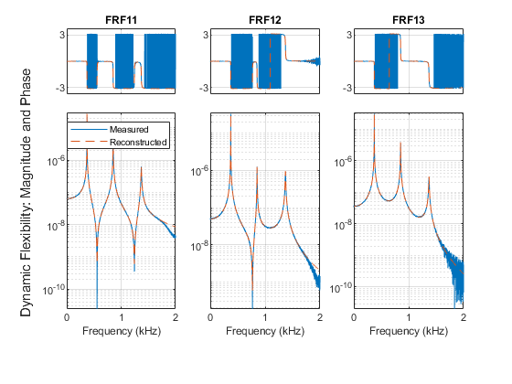
Estimate natural frequencies and damping and plot reconstructed and measured FRFs. Specify four modes and physical frequencies determined from the stability diagram, 'PhysFreq'. modalfit returns modal parameters only for the specified modes.
modalfit(FRF,f,fs,4,'PhysFreq',physFreq)
[fn1,dr1] = modalfit(FRF,f,fs,4,'PhysFreq',physFreq)
fn1 =

   1.0e+03 *

    0.3727
    0.8525
    1.3706


dr1 =

    0.0008
    0.0018
    0.0029
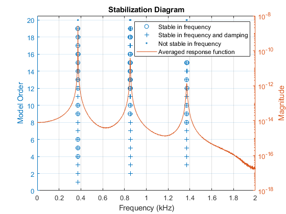
Next, compute FRFs and plot a stabilization diagram for a second set of hammer impacts with the sensor at a different location. Change the stability criterion to 0.1 percent for frequency and 2.5 percent for damping.
[FRF,f] = modalfrf(X2,Y2,fs,winLen,'Sensor','dis','Measurement','rovinginput');
fn = modalsd(FRF,f,fs,'MaxModes',20,'SCriteria',[0.001 0.025]);
With the more stringent criteria, the majority of poles are classified as not stable in frequency. The poles that are stable in frequency and damping align closely with the averaged FRF, suggesting they are present in the measured data.
physFreq = fn(4,[1 2 3]);
Extract modal parameters for this set of measurements and compare to the modal parameters for the first set of measurements. Specify the indices of the driving point FRF, corresponding to location where the excitation and response measurements coincide. The natural frequencies agree to within a fraction of a percent, and the damping ratios agree to within less than four percent, indicating that the modal parameters are consistent from measurement to measurement.
[fn2,dr2] = modalfit(FRF,f,fs,4,'PhysFreq',physFreq,'DriveIndex',[1 2])
fn2 =

   1.0e+03 *

    0.3727
    0.8525
    1.3705


dr2 =

    0.0008
    0.0018
    0.0029
Tdiff2 = table((fn1-fn2)./fn1,(dr1-dr2)./dr1,'VariableNames',{'diffFrequency','diffDamping'})
Tdiff2 =

  3×2 table

    diffFrequency    diffDamping
    _____________    ___________

      2.9972e-06      -0.031648
     -5.9335e-06     -0.0099076
       1.965e-05      0.0001186
A parametric method for modal parameter estimation can provide a useful alternative to peak-picking and the LSCE method when there is measurement noise in the FRF or the FRF shows high modal density. The least-squares rational function (LSRF) approach fits a shared denominator transfer function to the multi-input, multi-output FRF and thus obtains a single, global estimate of modal parameters [4]. The procedure for using LSRF approach is similar to that for LSCE. You can use stabilization diagram to identify stationary modes and extract modal parameters corresponding to the identified physical frequencies.
[FRF,f] = modalfrf(X1,Y1,fs,winLen,'Sensor','dis','Measurement','rovinginput');
fn = modalsd(FRF,f,fs,'MaxModes',20, 'FitMethod', 'lsrf'); % Identify physical modes using lsfr
physFreq = fn(4,[1 2 3]);
[fn3,dr3] = modalfit(FRF,f,fs,4,'PhysFreq',physFreq,'DriveIndex',[1 2],'FitMethod','lsrf')
fn3 =

  372.6832
  372.9275
  852.4986


dr3 =

    0.0008
    0.0003
    0.0018
Tdiff3 = table((fn1-fn3)./fn1,(dr1-dr3)./dr1,'VariableNames',{'diffFrequency','diffDamping'})
Tdiff3 =

  3×2 table

    diffFrequency    diffDamping
    _____________    ___________

     -7.8599e-06      0.007982
         0.56255       0.83086
         0.37799       0.37626
A final note about parametric methods: the FRF estimation method ('subspace') and the modal parameter estimation method ('lsrf') are similar to those used in System Identification Toolbox for fitting dynamic models to time-domain signals or to the frequency-response functions. If you have this toolbox available, you can identify models to fit your data using commands such as tfest and ssest. You can assess the quality of the identified models using compare and resid commands. Once you have validated the quality of the model, you can use them for extracting modal parameters. This is shown briefly using a state-space estimator.
Ts = 1/fs; % sample time
% Create a data object to be used for model estimation.
EstimationData = iddata(Y0(1:1000), X0(1:1000), 1/fs);
% Create a data object to be used for model validation
ValidationData = iddata(Y0(1001:2000), X0(1001:2000), 1/fs);
Identify a continuous-time state-space model of 6th order containing a feedthrough term.
sys = ssest(EstimationData, 6, 'Feedthrough', true)
sys =
  Continuous-time identified state-space model:
      dx/dt = A x(t) + B u(t) + K e(t)
       y(t) = C x(t) + D u(t) + e(t)

  A =
            x1       x2       x3       x4       x5       x6
   x1    4.041     1765   -149.8     1880   -49.64     -358
   x2    -1764  -0.3434     2197   -232.5    438.3    128.4
   x3    152.4    -2198    2.839     4715   -255.9   -547.5
   x4    -1880    228.2    -4714   -15.91     1216    28.79
   x5    59.42   -440.9    275.5    -1217    35.03    -8508
   x6    363.7   -120.2    545.4    44.02     8508   -92.47

  B =
             u1
   x1   -0.2777
   x2   -0.6085
   x3   0.07123
   x4    -3.658
   x5  -0.04771
   x6     7.642

  C =
               x1          x2          x3          x4          x5          x6
   y1   -4.46e-05  -5.315e-06   -7.46e-06  -1.641e-05  -2.964e-06   5.871e-06

  D =
              u1
   y1  7.997e-09

  K =
               y1
   x1  -3.513e+07
   x2  -3.244e+06
   x3  -3.598e+07
   x4  -1.059e+07
   x5  -1.724e+08
   x6  -7.521e+06

Parameterization:
   FREE form (all coefficients in A, B, C free).
   Feedthrough: yes
   Disturbance component: estimate
   Number of free coefficients: 55
   Use "idssdata", "getpvec", "getcov" for parameters and their uncertainties.

Status:
Estimated using SSEST on time domain data "EstimationData".
Fit to estimation data: 99.26% (prediction focus)
FPE: 1.355e-16, MSE: 1.304e-16
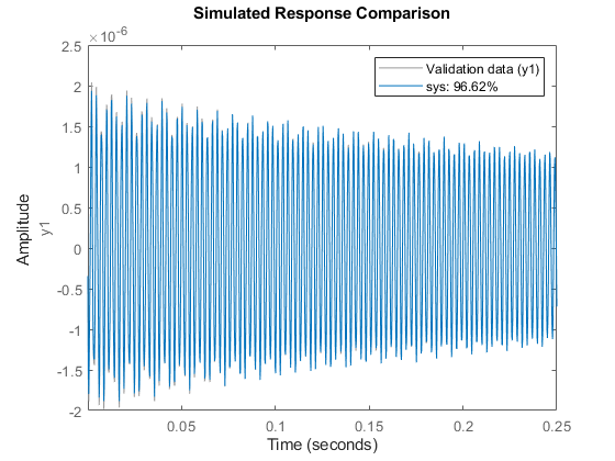
Assess the quality of the model by checking how well it fits the validation data.
clf
compare(ValidationData, sys)  % plot shows good fit
Use the model sys to compute modal parameters.
[fn4, dr4] = modalfit(sys, f, 3);
Mode Shape Vectors of a Wind Turbine Blade
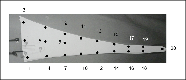
Understanding the dynamic behavior of wind turbine blades is important to optimize operational efficiency and predict blade failure. This section analyzes experimental modal analysis data for a wind turbine blade and visualizes mode shapes of the blade. A hammer excites the turbine blade at 20 locations, and a reference accelerometer measures the responses at location 18. An aluminum block is mounted at the base of the blade, and the blade is excited in the flap-wise orientation, perpendicular to the flat part of the blade. An FRF is collected for each location. The FRF data are kindly provided by the Structural Dynamics and Acoustics Systems Laboratory at the University of Massachusetts, Lowell. First, visualize the spatial arrangement of the measurement locations.
Load and plot the wind turbine blade FRF estimates for locations 18 and 20. Zoom in on the first few peaks.
[FRF,f,fs] = helperImportModalData();
helperPlotModalAnalysisExample(FRF,f,[18 20]);
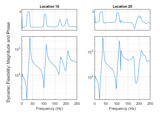
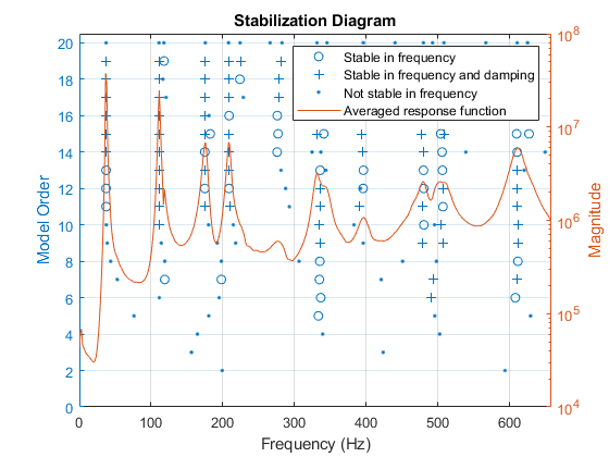
The first two modes appear as peaks around 37 Hz and 111 Hz. Plot a stabilization diagram to estimate the natural frequencies. The first two values returned for a model order of 14 are stable in frequency and damping ratio.
fn = modalsd(FRF,f,fs,'MaxModes',20);
physFreq = fn(14,[1 2]);
Next, extract the mode shapes for the first two modes using modalfit. Limit the fit to the frequency range from 0 to 250 Hz based on the previous plot.
[~,~,ms] = modalfit(FRF,f,fs,14,'PhysFreq',physFreq,'FreqRange',[0 250]);
Mode shapes quantify the amplitude of motion for each mode of a structure at each location. To estimate a mode shape vector, one row or column of the frequency-response function matrix is needed. In practice, this means that either an excitation is needed at every measurement location of the structure (in this case, a roving hammer), or that a response measurement is needed at every location. Mode shapes can be visualized by examining the imaginary part of the FRF. Plot a waterfall diagram of the imaginary part of the FRF matrix for locations on one side of the blade. Limit the frequency range to a maximum of 150 Hz to examine the first two modes. The peaks of the plot represent mode shapes.
measlocs = [3 6 9 11 13 15 17 19 20]; % Measurement locations on blade edge
helperPlotModalAnalysisExample(FRF,f,measlocs,150);
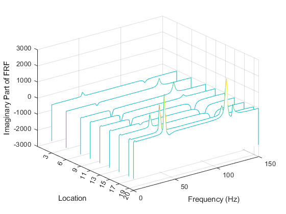
The shapes indicated in the plot by the contour of the peaks represent the first and second bending moments of the blade. Next, plot the magnitude of mode shape vectors for the same measurement locations.
helperPlotModalAnalysisExample(ms,measlocs);

While the amplitudes are scaled differently (mode shape vectors are scaled to unity modal A), the mode shape contours agree in shape. The shape of the first mode has a large tip displacement and two nodes, where vibration amplitude is zero. The second mode also has a large tip displacement and has three nodes.
Summary
This example analyzed and compared simulated modal analysis datasets for a 3DOF system excited by a roving hammer. It estimated natural frequency and damping using a stabilization diagram and the LSCE and LSRF algorithms. The modal parameters were consistent for two sets of measurements. In a separate use case, mode shapes of a wind turbine blade were visualized using the imaginary part of the FRF matrix and mode shape vectors.
Acknowledgment
Thanks to Dr. Peter Avitabile from the Structural Dynamics and Acoustics Systems Laboratory at the University of Massachusetts Lowell for facilitating the collection of the wind turbine blade experimental data.
References
[1] Brandt, Anders. Noise and Vibration Analysis: Signal Analysis and Experimental Procedures. Chichester, UK: John Wiley and Sons, 2011.
[2] Vold, Håvard, John Crowley, and G. Thomas Rocklin. "New Ways of Estimating Frequency Response Functions." Sound and Vibration. Vol. 18, November 1984, pp. 34-38.
[3] Peter Van Overschee and Bart De Moor. "N4SID: Subspace Algorithms for the Identification of Combined Deterministic-Stochastic Systems." Automatica. Vol. 30, January 1994, pp. 75-93.
[4] Ozdemir, A. A., and S. Gumussoy. "Transfer Function Estimation in System Identification Toolbox via Vector Fitting." Proceedings of the 20th World Congress of the International Federation of Automatic Control. Toulouse, France, July 2017.