Evaluar el número óptimo de clusters
Identifique el número óptimo de clusters en un conjunto de datos utilizando la función evalclusters.
Como alternativa, puede realizar la agrupación de k-medias de forma interactiva usando la tarea de Live Editor Cluster Data.
Cargue el conjunto de datos fisheriris.
load fisheriris
X = meas;
y = categorical(species);
X es una matriz numérica que contiene dos medidas de sépalos y dos medidas de pétalos para 150 iris. y es un arreglo de celdas de vectores de caracteres que contiene las correspondientes especies de iris.
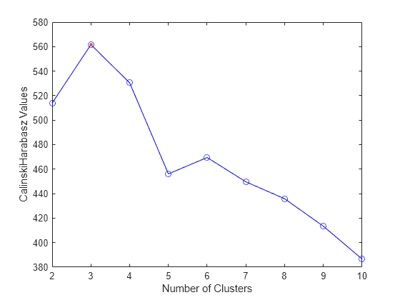
Evalúe el número óptimo de clusters de 1 a 10 usando el índice de Calinski-Harabasz. Agrupe los datos usando el algoritmo de agrupamiento de k-medias.
evaluation = evalclusters(X,"kmeans","CalinskiHarabasz",KList=1:10)
evaluation =
  CalinskiHarabaszEvaluation with properties:

    NumObservations: 150
         InspectedK: [1 2 3 4 5 6 7 8 9 10]
    CriterionValues: [NaN 513.9245 561.6278 530.4871 456.1279 469.5068 449.6410 435.8182 413.3837 386.5571]
           OptimalK: 3


  Properties, Methods
El valor OptimalK indica que, según el índice de Calinski-Harabasz, el número óptimo de clusters es tres.
Visualice los resultados de la evaluación de clusters para cada número de clusters.
plot(evaluation)
legend(["Criterion values","Criterion value at OptimalK"])
La mayoría de algoritmos de formación de clusters requiere conocer previamente el número de clusters. Cuando no se conozca el número de clusters, utilice técnicas de evaluación de clusters para determinar el número de clusters presente en los datos en función de una métrica específica.
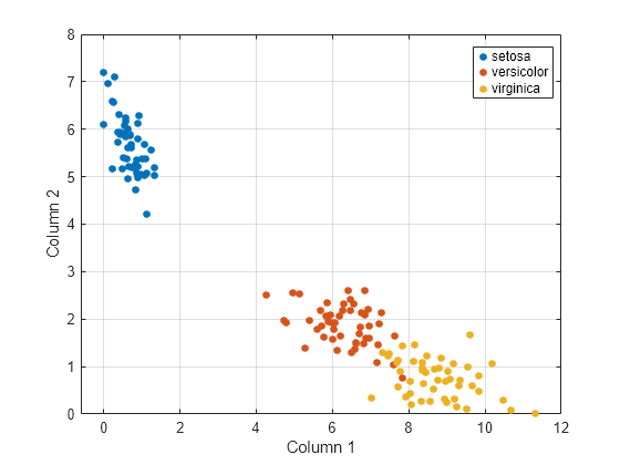
Tenga en cuenta que identificar tres clusters en los datos es consistente con que haya tres especies en los datos.
categories(y)
ans = 3×1 cell
    {'setosa'    }
    {'versicolor'}
    {'virginica' }
Para visualizar los datos, calcule una aproximación no negativa de rango 2 de los datos.
reducedX = nnmf(X,2);
Las características originales se reducen a dos características. Dado que ninguna de las características es negativa, nnmf garantiza que las características sean no negativas.
Visualice los tres clusters con una gráfica de dispersión. Utilice color para indicar las especies de iris.
gscatter(reducedX(:,1),reducedX(:,2),y)
xlabel("Column 1")
ylabel("Column 2")
grid on
Consulte también
evalclusters | nnmf | gscatter | Agrupar datos