Calibrating Optimal IPMSM Control Using Model-Based Calibration

Welcome to this MathWorks video. My name is Dakai Hu, and I'm part of MathWorks application engineering team. In this video, we are presenting a workflow demo slash exercise regarding interior permanent magnet synchronous motor torque and field-weakening control calibration. This topic is relevant to engineers working on electrification particularly those who are working on traction IPMSM drives.

In May 2021 we invited a GM technical specialist to talk about their use of model based calibration in their e-motor calibration workflows. You can watch the video clip of this talk at the conference proceedings on our website. As this model based calibration workflow is getting known by more and more motor control engineers, we received requests to show workflow demos or hands-on exercises that engineers can leverage as a short training session. That's the motivation behind making this video.

Before we start, I want to also point out that we published a technical article recently documenting some of the details of this workflow. For those of you who want to dive a little deeper, you can access this article by just typing the title into a search engine. I also want to use just one slide to explain what is MBC, or Model Based Calibration.

Model based calibration is a workflow for calibrating parameters for plant models and control systems. It includes steps for design of experiment, or DOE, model fitting and optimization, design parameter tradeoff studies, and calibration generation for lookup tables. Our goal of applying model based calibration workflow to electric motor calibration is essentially trying to calibrate field-weakening and torque control lookup tables.

There are primarily two types of talk control lookup tables. The first one is speed based tables. What that means is inputs to the table are torque commands and speech feedbacks. In order to account for bus voltage variation, we need to have multiple pages of these 2D look up tables. Each page here is calibrated based on a certain DC bus voltage. The second type of lookup table is the maximum flux based lookup tables. Here speed is used to calculate the maximum allowed flux linkage in combination with a feedback loop that involves the box voltage.

I'm not showing the complete control algorithm here, but the point is that inputs to the lookup table become maximum flux linkage and talk, and you only need one table for this algorithm. For the rest of this video, we will use the speed based lookup table calibration as an example and provide a hands on training and to walk you through the entire process. Let's get started.

In this exercise our example recalibrating the torque and field weakening control lookup table of an IPM motor that is about 120 kilowatts. I have the motor specs in here. So this IPM motor has eight poles, and the resistance per phase I believe this is around room temperature. And this is 0.01. The maximum speed we're going to calibrate is 10,000 RPN.

And the maximum current we are going to calibrate is up to 400 ampere RMS which translates to 565.7 Ampere peak. And for the DC bus voltage we're calibrating at 350 volts. Therefore, the maximum modulation voltage, VS max, we can calculate that based on this equation. Again, this differs from case to case. In our case, we can calculate that maximum modulation voltage is about 218.4 volts.

We're also going to take a look at the raw data. Here in this case, the DOE is already done, and the tests are also done. In this case, the raw table that you are looking at is basically the test data. So we have ID, and IQ, corresponding flux D and Flux Q the last column here is the measured torque.

The model based calibration toolbox doesn't accept the data format like this, so we have to rearrange it to a different format. What we are doing here is that we are using a simple script to read the raw table, and then we are doing some simple calculation to rearrange the table to a different format. So in the end here what you're looking at is a different table that has six columns, so torque, ID, IQ, and then speed, and then the corresponding modulation voltage which is calculated by the VDM DQ here, as well as the maximum current which is calculated by D and IQ.

So after running this, click Run, and this will generate a new Excel spreadsheet called IPMSN_MBCData. OK. That's the new data sheet generated. So you see that here we have six columns, torque, ID, IQ, different speed levels, and voltage VS and IS. So from here, now we are ready to import the data into the model based calibration toolbox.

Where can you access the model based calibration toolbox? If you install the model based calibration toolbox, you can go to apps, and then scroll down here, go to the automotive section. And you will find two apps. One is called Model-Based Calibration Model Fitting. And the other one is called MBC Optimization. So we are going to use both apps. And we'll first use the MBC Model Fitting tool. So let's launch that. With the MBC Model Fitting tool, the workflow goes from left to right. In our case, since we already have the test data, so we are going to skip the design experiment step. I'm going to go directly to the Import Data step.

Before that, let's create a new project. So click New Project. So that's created. And then click Import Data. The data in our case is coming from the Excel file. So click File, Open. And then it highlights the generated Excel spreadsheets, which is the IPMSM_MBCData.

Now the data is imported. I can find different ways to visualize it. I can look at it at 2D data plot or 3D data plots. So I'll click here and select 3D data. So I can look at, for example, speed-- actually Id, Iq. And choose speed as the Z-axis. It looks like in our raw data, we have the same data for each speed. We know that certain operating points are not achievable in the raw data.

So what we are going to do here is to create a filter or multiple filters to filter out operating points that are not achievable. To create filters, you can highlight here Filters. And then right click, Add filters. In our case, we know that we have voltage constraints and current constraints. So I'm going to highlight Vs, which is the voltage. And then this modulation voltage, we know that it has to be equal to-- or a smaller than or equal to the maximum, which is 218.4 volts.

So here I am going to add a 20% margin to that. And I'll explain why we need that later, if we have time. The same goes for current. So for current, we need this to be smaller than or equal to the maximum current, which is 400 RMS. And that is 565.7 peak. So times 1.2. Again, giving it a 20% margin. And click OK.

It looks like I've got a typo here. So 218.4. Now you will see that the data looks better. At least at high speed, the operating areas are smaller than the operating areas at lower speed. This is because at high speed, a lot of the Id, Iq operating points are filtered out. Because they either violate the voltage constraint or the current constraint.

Moving on from here, we can click Accept, the check mark here. So the raw data is now imported into the tool. We move on to the next step, which is to Fit Models. In our case, we are going to fit the Point-by-Point model. And the response in this case is Iq, and the modulation voltage Vs. The local inputs, we are going to use Id and Trq.

The operating point is speed. And we're also going to check this box, which is to use default models for large data. In our case, we have more than 10,000 data points after filtering even. So that's a pretty large data file. And then what we are doing here is once we check this box, the model fitting process will only fit one model, which in our case is the Gaussian process model, instead of fitting four different models to the data.

So from here, we click OK. You will see this window popping up. So what this window does is it allows you to group different tests into the same tests. For example, if your diano measures speed around 1,000 RPM, and the next set of measurement comes in at 1,001, 1,003, 1,005 RPM, and if you set this tolerance here to be 10, then what that means is that plus minus 10 RPM will be considered the same RPM testing operating point.

So all these 1,001, 1,003, or 1,005 operating points will all be grouped into the 1,000 RPM testing point. So in our case, we choose 10 as the Tolerance. And then check Sort Records Before Grouping. In our case, remember we are calibrating from 1,000 to 10,000 RPM and with increments of 250 RPM. So we ended up with 37 tests, or 37 operating points defined according to the speed.

So once we click the OK, now the tool will start the model fitting process. And this process will take approximately, in my case, three minutes. And this is based on your number of operating points, your number of test points. So I have over 10,000 test points. And then the time it takes to finish the model fitting is in direct proportion to the number of testing points cubed.

I have four workers on my laptop. And I'm using a Parallel Computing Toolbox, which is utilizing all four workers at the same time. And this will take, as I mentioned earlier, about three minutes. So in the video, I'm going to speed this up.

Now the model fitting process is finished. Let's take a look at what we get. So here we have two responses. One is Iq. And one is Vs. Click Iq. And these are the models. So for each operating point of speed, we end up with one model of Iq. So here we select a test. We'll see that different operating points are arranged here. And then we can highlight, for example, at this operating speed. And click OK. And this is the surface of Iq.

The same goes for Vs. Because for each operating point or speed, we have a Vs surface. You can also, if you like, right click and then Print To Figure, so that you can open up a formal MATLAB figure file to look at the fitted models.

Let's also look at an operating point that has high speed. So I'll choose a test that is very high-- has very high speed, let's say 9,750 RPM. And let's choose the Iq. You will see that the operating areas are greatly reduced compared with, let's say, a low-speed operating point. Select 1,000.

So you end up with a much smaller operating area on the Id, Iq plane at high speed. This is understandable. Because at a high speed, your voltage limit ellipse will shrink. And that will limit your viable operating region on the Id, Iq plane.

We are satisfied with the fitted models. Now let's save them first before we move on to the next step. Just a quick save. I'm going to give it a name. I'll call it FittedModels. This project will be saved into a .mat file. It looks like now it's saved.

Now we are moving on to the MBC optimization. We can open the MBC optimization app from here in the Apps section. Or we can just go into the model browser that we used to fit the models. And go to the top. And then open that from here. So Generate Calibration is essentially bringing up that MBC Optimization app.

This app is also called CAGE Browser. CAGE stands for Calibration Generation. Once you're in CAGE, first thing, it will ask you to import the models. So in this case, it automatically detects the models fitted from last step, which are the Iq and Vs models. So here I'm just going to click OK. And that will import all the models fitted from last step.

Now you're seeing that the models are inside CAGE. In this exercise, we're going to do two different types of optimizations. The first one is to calibrate the torque speed envelope under our specified voltage and current constraints. The second optimization is to calibrate the final torque and field-weakening control current to reference lookup tables for Id and Iq.

Let's get started with the first optimization, which is to find the torque speed envelope. To do that, first we have to create a function model. And this is for current, Is. So remember we had Is previously in the raw data. But in this exercise, we didn't fit Is model. We didn't have to. Because we can calculate easily, Is, from Id and Iq.

So in this case, we're going to do that. Is equals square root of Id squared plus Iq squared. Next. And Finish. We also need to create another function model called TrqModel. So I'll give it the name TrqModel. And this will simply equal Trq. The reason why we need a TrqModel is because we need a model so that we can run optimization to either maximize or minimize.

In this case, we're going to maximize TrqModel at each operating point of speed. So those torque operating points, the maximum torque operating points at each speed point will constitute the final torque speed envelope. Click Next. And Assigned Input automatically assigns the original torque as the input. And we're going to click Finish.

After creating the two function models, before we can create an optimization, first we need to create a table that contains all the optimization points. So we're going to go to File, New, 1D Lookup Table. And I'm going to call it TrqEnvelopeTbl.

I just lagged to speed. Speed is the table operating points. And we're going to go from 1,000 to 10,000. In this case, we have-- remember, initially when we grouped the tests, we have 37 tests. So just put 37 here. These are the operating points that will hold the final optimization results. We're starting at 1,000 RPM. And it goes all the way to 10,000 RPM at increments of 250 RPM.

Now we have prepared everything. We're just going to go to Optimization. And then from here, Create an Optimization. In this optimization, we'll go into maximize TrqModel. So highlight TrqModel. Click Next. And then select here Maximize. You can choose different algorithms for your optimization.

In our case, the default is fmincon, which is the most commonly used local optimizer. And for certain cases, you can choose to use a global optimizer if you have installed the Global Optimization Toolbox, things like pattern search or genetic algorithm.

Now we can click Finish. At this page, we work from top to bottom. On the top here, the objective is already set up. So we're trying to maximize TrqModel. And then we also need to tell the optimizer what the constraints are. In our case, we have two constraints, current and voltage. So the current has to be smaller than or equal to 565.7 amperes. This is the peak phase current. Click OK.

And the voltage has to be smaller than or equal to 200-- I believe it's 218.4 volts. And this is the phase modulation voltage. What we also need is to add a boundary model. So remember when we create the models, we have the Iq model and the Vs model. We have to select either one. And then here, choose the Boundary Constraint.

Because if we don't select the model boundary as a boundary constraint, then the optimizers may search areas that fall outside of the model boundary. Now we have set up all the constraints. And the last thing we have to do before we run the optimization is to set up the three variables and fixed variables. The fixed variables are essentially the speed operating points. And then free variables are Id and Trq.

What we can do is go to Optimization. And click Select Variable-- or Select Free Variables. And select Trq and Id as the free variable. And leave the speed blank. So that speed will be automatically selected as the fixed variable. By default, there's only one operating point. We need to import all the operating points we want to run for optimization.

So we have to go right click and then select Import From Lookup Table Breakpoints. And select TrqEnvelopeTbl, which has 37 operating points of speed. So now the 37 operating points are imported in here. From now on, what we need to do is simply just click a button, Run. And that will basically kick off the optimizer. And the optimizer will search on the response surface, trying to find what the maximum torque is at each operating point.

Again here, I'm relying on the Parallel Computing Toolbox. And I'm not speeding up the video. So because this process is relatively fast. It takes less than one minute to finish the entire optimization. It looks like now it's done. So this is the final optimization results. I can obviously pop it up to a formal MATLAB figure. And then this is the torque speed envelope that we optimized.

And then from here, we need to fill these optimization results to the tables that we created. Well, one table only, the TrqEnvelopeTbl. So we click Fill Lookup Table. And highlight that TrqEnvelopeTbl we just created. And then fill that with the optimization results. Click Next. And there are different filling methods. In our case, Direct Fill. There's no extrapolation or interpolation going on. So this is the final table that we are looking for.

We are now done with the first task. Let's move on to the second task, which is to create an optimization to get torque and field-weakening control Id, Iq lookup tables. We will have to rely on this torque and speed envelope to create the TrqGrid used for generating the final lookup tables. Because in this exercise, we want to use the percentage of maximum torque instead of absolute torque values for the lookup tables.

To do that, we have to first create a torque envelope model, which is essentially a math expression of this torque speed envelope. So let's go to Table. And click Convert to Model. And click OK. Actually, you can name it. Instead of the original TrqEnvelopeTbl, we can change the name here. Just call it TrqEnvelope. And click OK.

Now you'll see under the function model section here. Now there's a model called TrqEnvelope being created. You can actually see what the model looks like in the lower right corner here. Once we have the TrqEnvelope model, next step is to create another function model named TrqPct. So click New Function Model and type TrqPct.

This function model is calculated by the original torque from the raw data and divided by this TrqEnvelopeTbl or model. And then times 100. Click Finish. With this new function model called TrqPct, now let's create a table based on this torque percentage.

So we can go to Tools, Create Lookup Tables from Model. Then click Next. Here we have to select speed as the row input and TrqPct actually as the column input. For the speed, the normalizer is the norm speed, which we created earlier. So starting from 1,000 all the way to 10,000 RPM with increments of 250 RPM.

For the TrqPct, we have to create our own grid. So in this case click this button. And then we're going to use a Freeform Vector starting with 1% and then 4%, with increments of 4, and all the way to 100% of maximum torque. The reason we don't want to start from 0% is because when the torque is 0, there's no way the optimizer will be able to find a single operating point that can satisfy this objective to achieve the maximum of efficiency or TPA, which we'll explain later.

And therefore, here we-- instead of using 0, we use 1% of the maximum achievable torque. Click OK. Then click Next. And then now the table is created. Now let's go back to the Models tab. We still have to create another function model named TrqGrid. TrqGrid is the absolute torque calculated by torque percentage and the torque envelope.

So here let's go ahead and Create a New Function Model. And then type TrqGrid grid equals TorqPct-- actually, a TrqPct input. This is an automatically created variable once we create the TrqPct. TrqPct_input is essentially a number from one to 100 that represents the percentage of maximum torque.

So in this case, TrqPct_input divided by 100, that gives us the actual percentage. And then times the TrqEnvelope. So this is the TrqGrid. Click Finish. From here, we have done all the preparation work. We created all the variables needed. We created all the function models needed.

And now the last thing we need to create is called TPA. So this is torque per ampere. And it's used as the surrogate to indicate efficiency. So a TPA is calculated as Trq divided by current. Here Trq is actually indicated by TrqGrid. Because TrqGrid is calculated by the absolute torque percentage times the TrqEnvelope. So that's why we replaced the original torque with the TrqGrid here.

What we also have to do is to replace the torque inputs for the original Iq model, as well as the original VS model with TrqGrid, grid, which is the function model we created. So here we highlight Iq and click Edit Inputs. And then highlight the Trq. And use TrqGrid to replace that. We do the same thing with the Vs. Edit inputs. And replace with TrqGrid.

And finally, the last thing we have to do before creating the optimization is to actually create the Id, Iq lookup tables that are used to contain the optimized table data. To do that, we highlight Iq. And go to Tools. And select Create Lookup Tables from Model. And click Next.

Here, obviously, the speed is used as rows. And TrqPct is used as the columns. So here select speed norm and TrqPct_norm. So you can see the grids for speed, the same one as before from 1,000 to 10,000 increments of 250. And then for the TrqPct from 1% all the way to 100%, starting from the second, increments of four.

Click Next. Create Lookup Tables for Id and Iq. Click Finish. Now the tables are created. Now let's go to Optimizations. So click here to highlight the original project, top of the project tree. And then click Create Optimization. What we're trying to do is we're trying to maximize the TPA. So highlight TPA. Click Next. Click Maximize. Click Finish.

When we are at this page, we're following the same workflow as before. So work from top to bottom. We have the objective set up, which is to Maximize TPA. And then we're going to add constraints. So it comes with TPA boundary constraints. What we also have to do is to create the voltage constraints and the current constraints.

For voltage, the constraints is that this voltage, Vs, has to be smaller than or equal to 218.4 volts. And then for the current constraints is that the current, Is, has to be smaller than or equal to, I believe, 5-- 65.7 amperes. This is the peak one.

What I also want to add is to add the original boundary of Iq model. So click Iq. And here we're going to select Boundary Constraint. Remember the optimizers cannot go beyond those model boundaries to search for optimized solutions. Now let's work on the optimizations point set. This is basically your operating points. So we have the Trq and speed grid. Therefore, the fixed variables are torque percentage and speed. And the free variables are basically just Id.

So we can go to Optimization, Select Free Variables. We select Id. And then automatically, the fixed variable here becomes speed and TrqPct. But here it's only 37 operating points. We have more than that. We have a number of speed operating points times a number of torque operating points. Actually, we have to import that from the tables. Right click here. And then click Import From Lookup Table Breakpoints. In this case, either Id or Iq_Table. They're the same.

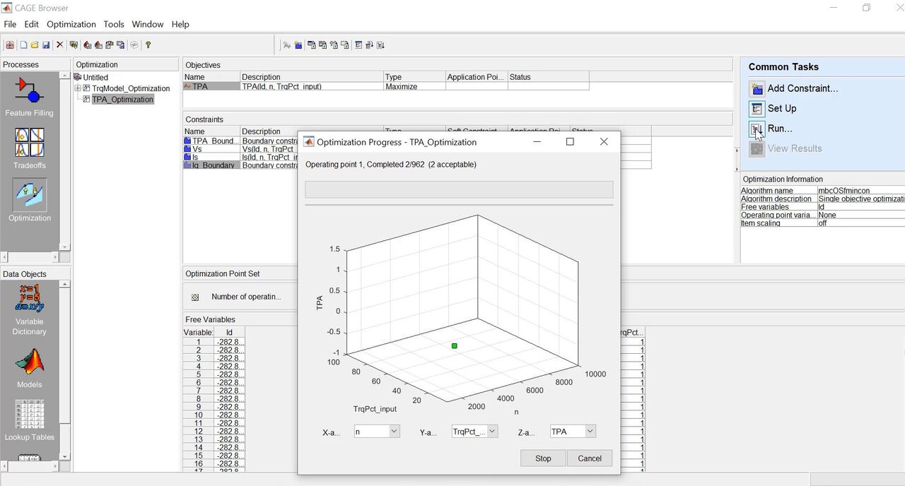
So altogether, we should have 37 times 26 operating points or fixed variables. And you see the number now becomes 962. At this point, I believe we prepared everything to run this optimization. So all we have to do is go here. And let's click Setup. Instead of starting from one point to run the optimizer, what I prefer is to always start from three points. This will give us a better accuracy.

So let's click Run. Depending on your PC, this process can take somewhere between less than one minute to a couple of minutes. In my case, I have 962 operating points. And I'm using a full core PC running Parallel Computing Toolbox. And it will take roughly around three minutes. So for the sake of this video, I'll just speed up the process here.

Now the process is finished. And you will see that we have 962 operating points. And all of them, we were able to find acceptable solutions. So each green dot indicates that the optimizer was able to find an optimal solution. We can right click here and then Print to a MATLAB Figure. So you can take a closer look at it.

Now we have the optimization results. The last step here is to fill in the tables that we created earlier. So the Id and Iq tables. Actually, the Id_Table is already here, that you're looking at. And then Iq_Table, we need to fill that from here. So Id_Table, Iq_Table. Click Next. And Id, Iq, Fill With Id, Iq. And then the Normalizer, which is the inputs for the grid. So the speed and then TrqPct.

Click Next. In this case, we're still going to use a Direct Fill. Because we don't want to extrapolate or interpolate. Click Finish. You will see the results here under table section. So right here. And click Lookup Tables. And click-- this is the Id_Table. If I click Iq, this is the Iq_Table.

So I can also right click Print to Figure. As you can see that now on the x-axis, this is speed. So starting from 1,000 to 10,000 with increments of 250. And then on the Y-axis, we have TrqPct. So for 1% all the way to 100%. And this is based on that torque speed envelope, which means that at 10,000 RPM, that operating point corresponds to a different absolute torque compared to, let's say, 2,000 RPM. Even though there's 100%.

But this 100% is based on the maximum torque achievable at 2,000 RPM. And then this TrqPct is based on the maximum torque achievable at 10,000 RPM. So by filling the table in this manner, we make sure that each operating points are viable operating points. There are no operating points wasted. Let's actually take a look at the Id_Table as well. Click Id. And let's Print it to a MATLAB figure.

So on the Id_Table, we can clearly see that here, if I rotate it this way, you will see that as speed increases, first you'll see this flat area, which basically is below base speed. And this is MTPA trajectories. And then once your speed increases beyond base speed, you'll see that in order to maintain Trq, in this case, when speed increases, Id increases in a negative direction. So along this line here. First MTPA. And then increase Id to the negative direction as speed increases.

So overall, this area is the field-weakening area right here. Now it looks like we're done with our second task. We already got lookup tables for Id and Iq. The last thing we want to do, if you want to export calibration lookup tables, you can do that from here. You can go to File. Go to Export, Calibration. And you can export the Id, Iq_Table as well as all the other tables we created.

In this case, let's say we only care about Id and Iq_Table. And obviously, we need the TrqPct_norm, which is the inputs of the TrqGrid and as well as the speed grid. And we can do different file formats. Let's say we want to do a Simple CSV File. And give it a name. CalibrationLuT_Id_Iq.

Now the table is created. You look in here. You can open it outside MATLAB. Now this is just the indices for the inputs. And then this is the Id_Table. And I think below here is the Iq_Table. Let's see what it looks like if we plot it here in Excel. Let's highlight the data. Let's do it for Id_Table.

And just go to Draw-- actually, Insert. Go to the Charts. Do a Surface Chart. So you'll see the same surface as you see in the CAGE Browser. The difference is that here, you cannot really rotate very well. Now we completed both tasks. We ended up with two calibration tables. We need the Id_Table and Iq_Table that has both the torque control and field-weakening control lookup table data in it.

So this concludes our exercise. Thank you very much for watching. And I've written down my email here, dakaihu@mathworks.com. If there's any questions regarding the model-based calibration process or just electric motor calibration in general, please let me know and I'll be happy to help.