Design and Commissioning of Robots in Smart Factory

Today we will be seeing a webinar on design and commissioning of robots and smart factories, et cetera. I am your speaker, Ramanuja Jagannathan. And I'm an application engineer from MathWorks, who primarily works in the area of control design. This webinar today is part of the smart factory webinar series, which has been happening since yesterday.

So today we'll be looking into robotics, design and commissioning activities. Do join us tomorrow. I will be talking more on the deploying of the autonomous algorithms and AI algorithms in smart factory set-up.

Let me start by putting a poll question to you, to understand where you are in your robotics journey. So you should be able to see a poll question come up with here. So you can let us know where you are in the journey. Maybe you are working in a project activity, or you are looking to work in a project in the next two to three months.

Or you may be here to understand what's happening in robotics and to build your competence. Do fill out this poll so that it helps us understand where you are in your journey. So you would still have some time to answer that. So please do answer that.

And while you answer it, I can give you a brief of what we'll be covering in today's webinar. We will definitely be touching upon how to design robotics in industrial setup, what's happening in industrial robotics, what are the trends today. All right, so let me start with some of the trends which happen with industrial robotics.

Now we see this trend technology creating a new wave in manufacturing technologies. We've seen a lot of assets being connected, and data from these assets are used to create smart value chains and to optimize the entire production process. We also see a lot of AI based and flexible robots being put up into this setup, where they're connected digitally and increase intelligence.

The concept of smart factory has been promoted in recent times, owing to the digital transformation. Now this concept leads to optimize the overall assets, operation, and workforce in your factory. A lot of data is collected from your IoT systems, which help to extract intelligence from these machines. And you would be able to create intelligence and optimize the overall production process.

Autonomy has been introduced into smart factory, so that you could work in a more safer environment with increased productivity. Definitely, the smart factory setup is going beyond the normal automation. Here, you see advanced robots, such as cobots and AI-enabled robots come into the picture, who credit to the increased complexity of smart factories. And AI and data analytics help these robots work more reliably.

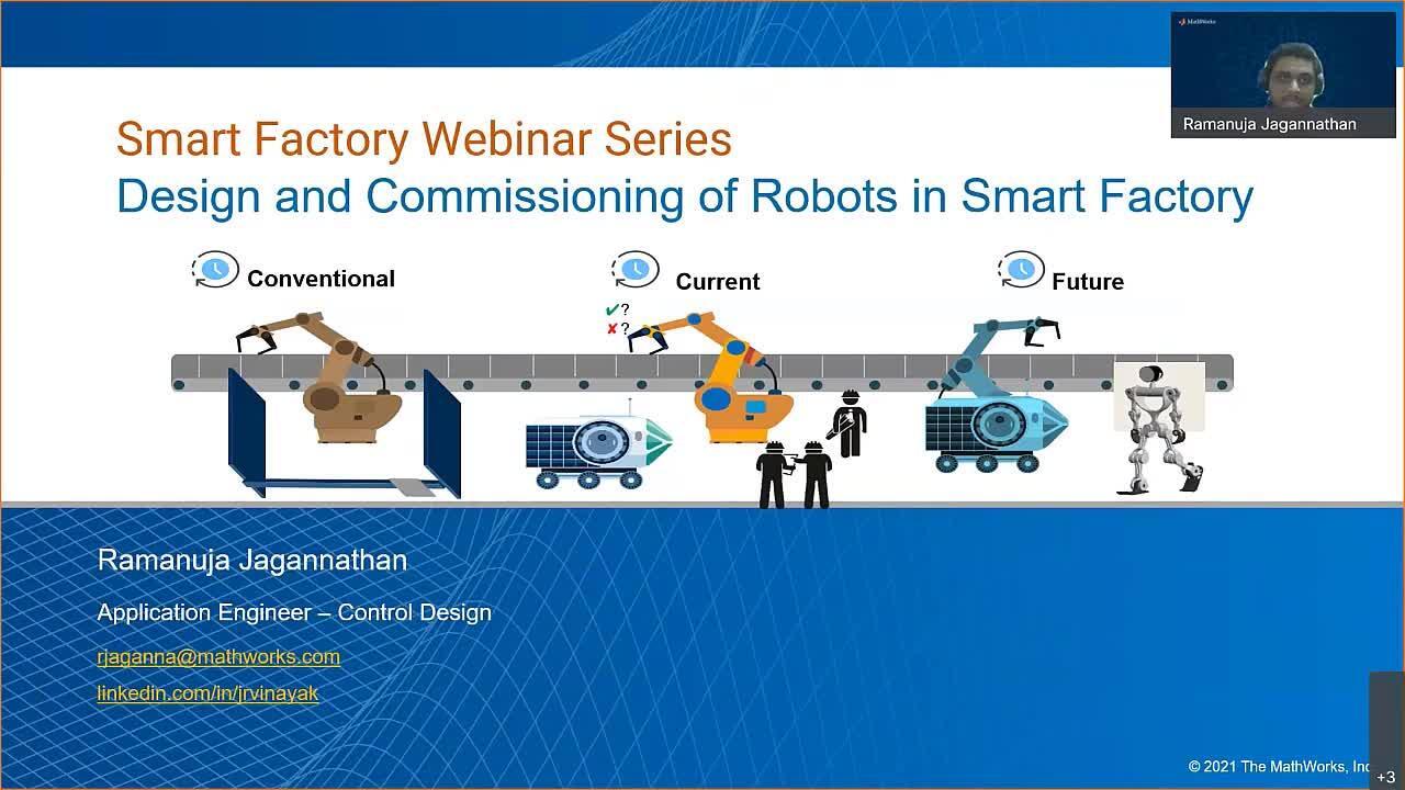
Now, let's look into some of the trends which we see with the robots in smart factories. The conventional robots are the ones who can perform repeated tasks very quickly. These robots are manually programmed, and since they can't sense the environment, they need to be fenced to keep a safe workplace. One example is from Mitsubishi.

While they build their robots using model-based design with MATLAB and Simulink, they build controls for their robots which meet accurate requirements and stringent conditions. Now, we can increase more productivity when humans and robots interact with each other. Now that's where you see the cobots or collaborative robots enter the smart factory space.

These robots perform typical tasks, such as the pick and place, painting, packaging. They are easy to program and deploy. And since they can perceive the environment, it's more safe to work with these robots. Finally, we are able to bring safety and increase productivity with these robots in a factory workplace.

One example is from Yaskawa who makes pick-and-place robots which have perceptual abilities, such as voice given commands and video perception abilities, which helps it in performing part planning and controls activity. But the true objective of autonomous systems is to make its own decisions autonomously and not programmed. Now that's where AI-driven robots come into picture.

Now, these robots have advanced perception and planning algorithms put into them. They interact with the environment and learn from those interactions. And they're able to adapt to complex scenarios and work more human-like. One example of such robots is the Agile Justin robot from DLR.

This robot has stereoscopic vision, tactile sensors, and can perform human-like activities. DLR used model-based design with MATLAB and Simulink, who develop and test and deploy these autonomous algorithms. When we built these robots, there are, of course, multiple challenges. Now, these challenges come from two main concerns.

One is the increasing complexity of our devices. Increasing complexity mean that there's a lot of multi-domain expertise required to build these systems. You might need to know autonomous algorithms, computer vision, artificial intelligence, and mechatronics.

Another complexity is in developing the software for these components, mainly how complex robots, such as cobots and AI-enabled robots, which come up with intelligence and connectivity, the number of features they were, definitely that increases. So how do we tackle these challenges? That's what we're going to see in today's webinar.

And the agenda for the webinar would be to talk about how to develop such robots, starting from the conventional robots, build the AI-based robots. But when I talk about conventional robots, we typically talk about the actuator requirements. We talk about control design and how to commission that.

And when we come to the autonomous robots, there's more talk about how to include autonomous robots into them. So we will take these two phases and cover the topic. So first we will start by developing an automatic robot. A company will be trying to develop a robot which can pick a payload from one conveyor belt, and it can drop it in another conveyor belt.

But the biggest challenge with such a robot is, you might want to know what actuators to choose and how to design the controllers. A typical way to do that would be to use simulations to get actual requirements and validate your control logic. We would follow the five-step process mentioned over here to develop such robots.

The first step is to import your CAD model. Now you could import CAD models from several softwares into Simscape Multibody. Now these CAD models bring in the mass, inertia, geometry, and joint details from these tools. Your CAD model could be imported using simple MATLAB commands, and once the import is done, you would see a multibody assembly pop up.

Now these models are useful to simulate a 3D CAD model what we designed. You could visualize the CAD model, and you will be able to simulate that, providing some actuation at joints. The next step is to add contact forces to these robots. Why would you do that? Because the robot has to interact with the payload.

Payloads may interact with each other, and the load may interact with the surfaces. Now, Simscape Multibody comes with spatial contact for blocks, which helps you interact with several geometries, such as point loads, bricks, cylinders, and spheres. If you don't have a CAD model with you already, you can use the standard models available in File Exchange.

Now these are models of the most relevant robots available at market today. Once the CAD model is imported, the next step is to subject it to various conditions and simulate for part group requirements. So here we would simulate the robot, with different load conditions, different speed, different friction levels, and at the full range of operations.

Now, these simulations give us the maximum torque which could be expected at a particular joint motion. Now, we use this information to select the appropriate motor, which could provide such torque limits. But once the motor is selected, the next step is to include that motor model into your simulation environment.

Here is where I could add motor models from Simscape Electrical Library into the CAD models. These motor models actuate the joints, which makes the robot move about itself. Well, these motor models are parameters from the data sheet. And here you could see that, how there's a correspondence between the parameters in datasheet and the parameters for the simulation model.

Now, once the mechatronics model is built, now we can go ahead and then try to build a trajectory. Now we want the robot to start from one position and then drop the payload at a different position. Well, this can be achieved by going through different trajectories.

How do we choose the optimal trajectory? We can probably minimize the power consumption, while moving from point A to point B. And how to find the trajectory with least power consumption? Basically, we perform dynamic simulations, and run optimization algorithms to determine the trajectory.

Now, here you see there are several points in the trajectory that we tune, so that we get more optimal power consumption. Rule that we definitely do multiple simulations. So here you could see that the robot is definitely trying to explore multiple trajectories. And on the right side, you'll notice that we're estimating what are the power consumption savings.

After a while, you would see that it converges to around 83% pace, meaning that we are getting 17% savings. And once we get that particular trajectory, we could take that for further control design. So here is a difference between the original trajectory, and then the power optimized trajectory. We can also try this trajectory with different parameters, such as different friction parameters, and then see how the system responds for each of these values.

Now, in the previous step, we did several simulations, right? Now doing several simulations means that it is going to take a lot of time, and it will be good to accelerate the computations. So that's where we can employ parallel simulations to enhance different computations. We could leverage different code level PC, or we could leverage cluster computers, where the work could be offloaded.

So once a trajectory is found, the next step is typically to design our control logic. The control logic starts by designating the variables which you want to sense. And these variables would trigger some actions in the robot, which you will define using a state chart. And then these state charts will give output to the robot.

Now, in this case, I have the conveyor, and once the payload reaches the conveyor, I want to trigger the robot action. So to check this, I have some logic, will check for whether the payload reaches the environment. And I have some sensor logic that checks if the payload touches the conveyor. Once you've got payload drops on the conveyor, next the straight shot triggers, and you could see that the conveyor started rotating, and then the robot started picking up the payload once it reaches the end destination.

So this state machine logic can be designed using state flow. So here you see that different events trigger state transition, and each of these state transitions decide how the robot should operate. Now similar logic can be designed for your gripper logic, when to open and when to close.

You can also define similar logic for their overall robot motion, that is, a robot moving from home position to the pick-up position, and then the drop-down position. And you see that these logics are interconnected by overlapping events. But once the control logic is done, the next step is to actually go and commission the controller with the robot.

Now here you would program, let's say, a PLC, and then connect it to the robot. And then you have commissioning and then see if everything works fine. Now what happens here is that you're basically testing the entire, you're basically delaying the testing process to the last phases of your commissioning activity. Now, you could be more intelligent and test your control logic with your virtual plant model.

Now what this leads to is to test your control logic even before commissioning, and to find out any errors before commissioning, so that you could go with a more quality product. If you're able to do modeling right from the beginning of the robot design stages, you could also design control logic, optimize it using models, and then integrate that with your actual target PLC. Now here, I will show you what are the steps to combine model-based design and virtual commissioning.

So the first step is that, in model-based design, you do model your plant, and then you do model your controller. And you perform alternate route test to see that the controller works fine. So here we designed the controller using state machines. And then we made the robot model.

Now I can perform dynamic simulations to understand how the controller interacts with the physical model. Here, I could see the active states, in the states of being active. And this helps me to debug my state flow, if at all I find some error in operation. So, once the desktop simulation phase is done, the next phase will be to generate a PLC code from the control model.

But that can be done using PLC coder, which can convert your Simulink model into a structured text. I will be covering the code generation process in tomorrow's session. So please join the session to understand more. But let's assume that the code got generated, and let's go on to the next step.

The next step is that we deploy that code into an actual PLC or PLC emulator. Once the code has been deployed, next we basically do a code simulation between the target PLC and then the plant model. Now this helps us to find out any error in the code, even before actually commissioning with the original robot. Now these are the steps which we take to actually commission your PLC. And once you are done with these steps, you can be more confident that your PLC is well designed, and it would mostly work on the day of commissioning.

So what are the other benefits of virtual commissioning? One benefit is that you can develop more optimal algorithms. You can explore different plan designs. If you start by designing your robot model right from the day one, you could improve the overall system level design. You could definitely target different PLCs or FPGA for embedded platforms with the same algorithm.

And the plant model, what you develop, could be used as a training simulator, once the process has been deployed, commissioned, and you want your operators to get trained on it. So one example I would like to touch upon, is from Krones, who develop the package-handling robots. Now, they used tools like Simscape Multibody to make their plan models, and test their control logic.

Now this helped them to be confident that the controller, what they designed, will actually work when they do the commissioning with the machine. Now here are some more resources for you to understand how virtual commissioning works. The resource on the left talks about how we can do virtual commissioning for a retention mission, and how to deploy a logical B&R PLC.

On the right, you'll see the virtual commissioning steps for the robot model, what we saw right now, and how we can deploy the model to a Siemens PLC. Of course, there are more links, which I would put over here, and then it will be shared to you later. So, we showed how to develop the platform, and how to design controls and test it and deploy that. Now, let's go to the next step of where we will include more autonomy into your robots.

At this step, I'll be talking about how we can build up robot models, build environment models, build autonomous algorithms, test it in these environment models, and then deploy them to your robot ROS model. So when we talk about autonomous robot development, there are three pillars which we want to think about. The first pillar is definitely on the platform design, which talks about the robot modeling and the environment model.

Once the platform is done, next, we would add some autonomous algorithms to that. So here, we talk about algorithm for perception, planning, and control. Once these algorithms are designed and tested with the environment, next, we would want to deploy these algorithms to either ROS nodes or through the platform robot. So that's where we talk about the deployment choices.

When we go through the development process, an ideal tool, which helps you in development, will have facilities to design, simulate, analyze, implement, and test your autonomous logic. Now, let's see how MATLAB and Simulink can help you in doing this. So let me start with the platform design. So just now we saw how, in Simscape, we can import your CAD model into Simscape Multibody.

You also saw how to improve actuators and connect them to the CAD model. Of course, there are other ways to import your robot models. Say, if you have a URDF file, you can import that using a single line of code. You could also use the in-built robot repository, and then choose the robot of your choice, for which you want to develop autonomous algorithms.

Once you develop the models, definitely you can try to simulate these models in your simulation platform. So, generally, what happens is that you might want to test your autonomous algorithms in your actual physical robot. And this could be sometimes time-consuming, expensive, or sometimes really dangerous. So what you do, is that you use simulations as a replacement for physical experimentation.

When you decide to go for simulation, there are different fidelities at which you could simulate your robot and environment. Now it's possible that each of these different fidelities are being done in different tools. Hence, you might want to start with the lowest fidelity, build your model, refine the model, and then incrementally add more details to that, so that you reduce the overall risk of development.

So let's see an example of how we go from low fidelity to high fidelity simulations. So here, we see an example where we want to perform task scheduling. Now task scheduling is typically the first step what do you do when you go design your robot algorithm. And for such an algorithm, you might use some interactive inverse kinematics tools. Or to simulate, to visualize the motion, you can actually use some simplified motion models.

Well, these simple models help you iterate your experimentation of task scheduling. And it helps you in defining better task scheduling algorithms. Now one thing what we don't simulate here is the actual grasping motion of your robot, and the dynamic actions of the robot.

As a next step, we could include that. Let's say I want to go one level higher, and I want to add controls to my autonomous system. So at this particular step, I could include robot models which actually simulate the robot dynamics. And it takes in torque commands and gripper commands as input.

Now these models, you can see that they are dynamic simulations actually. And you need to give in the torque command, which is actually making the robot move. One more level of fidelity is that you could also simulate the payload which the robot is going to lift. So here, we put into the multibody simulation what we discussed a few slides back, and that helps us adding the load dynamics also into the robot.

So here you could notice that the robot is actually able to pick the load, and when it picks, the dynamics of the load is also getting added, and the control system need to take care of that as well. Now here we simulated the robot dynamics incrementally. But let's say if you want to make the robot interact with the environment, then you can go ahead and then connect the robot models with third party simulation tools.

So here you see the Simulink model, which has the robot model communicating with Gazebo environment, while it is able to perceive the environment. Robotic system tool box also lets you perform time synchronized simulations. But you could see that the Simulink model and the Gazebo environment are equally based up.

But let's say if you want to have a more photorealistic simulation, and if you want to have a higher fidelity simulation, then you could also couple the simulation with targets like Unreal Engine. Now here you could see that the robot operating in this environment, and this looks more like a real factory setup.

Now let's go on to the next pillar of autonomous system design, where we will talk about the autonomous application designs. So let me first talk about how deep learning can be used in developing these autonomous algorithms, specifically for perception. Now there are robots that need to acquire audio signals and then interpret tests out of that.

Now these robots are driven by voice commands. And this is one characteristic of any cobot robot. Images also help us in understanding the environment better. So with images, we can actually identify the parts in the environment. And if there are going to be any anomalies, the robots could detect them as well.

Another mode of input is some point cloud processing. Point clouds could help the robot understand the 3D environment around it, so that it can localize itself, and then estimate the pose of robots. While the example I'll be talking about is primarily on the identification and detection of parts using vision systems. Now in this particular example, the robot is trying to scan the environment or the objects at different angles and different ambient conditions.

Here we create around 400 plus images, and these images are then fed to an labeling app which auto labels these different components. Once the labeling is done, the next step would be to print a deep neural network algorithm, and then classify and detect these parts. Once deployed, you could see how the robot perceives.

The left top view is the camera view from the robot. The left bottom view is how the robot perceives the environment, where it is able to correctly identify the mug and the membrane. And once it's identified the membrane, you could see that it is actually going to pick that particular object.

Now this leads me to talk about how a robot is actually planning to pick the object. So here's a complete workflow of the pick-and-place robot. The first step is the robot wants to scan and build an environment model around the robot. Now this is really useful, and there's a distinction between the conventional robots.

For example, let's say we have a dynamic environment, where the obstacle changes, right? The robot needs to perceive that, so that it could replan its motion. Also, if the robot is presented with different types of objects to be picked and placed, then it needs to understand them as well.

The second step is that it performs the perception process and identifies and predicts the objects. So this is the step what we just saw right now. So let me go on to the next step, of where we will talk about the pick and place workflow. But before going to that, I would also like to point to you some examples which are available in the software, which goes through the entire process what we're discussing right now.

So please explore these examples to get acquainted with the process. And when we talk about the pick and place workflow, it consists of two parts. The first part is path planning, and the second part is the trajectory generation. So when you perform path planning, the idea is that you want to create a waypoint, which basically avoids all obstacles and negotiates with the complex environment around it.

This is purely a geometry task, and when you get geometry coordinates at the end of this exercise. Now these points go to trajectory generation, where it gets a time association. So based upon constraints like position constraint, velocity constraint, and acceleration constraint, we put a time stamp to these waypoints, using some polynomial builds or velocity profiles. Well, let us look at one example over here.

But the robot, what you see over here, is basically able to navigate from this pick position to the drop position, by overcoming the obstacle. Now here, you see the way points which the robot takes to move from one point to another point. Here you see a heuristic value called maximum connection distance, which is kept at 0.5 right now.

And when this value is lower, typically what happens is that the robot chooses a shorter path, but it takes more time to compute such path. So you could play around with such heuristics, and then defend your waypoints. By the way, this waypoint was generated using a bi-directional RLD algorithm. Now, it could be the case that you are trying to control your robot in a new environment. Or the robot is given a very complex task to pick up a very new object.

So what to do in those cases? You could actually use reinforcement learning to train the robot under such different circumstances. So here we see that the robot is getting trained to pick up the cam. The input to the training algorithm is the current state of the robot.

And after a few iterations, you'll see that the robot will be able to pick the cam appropriately. And while this training occurs, we'll reward the algorithm, if the robot is able to properly pick the cam from its position. Another example is where we train the robot to pick up objects at different post conditions. So here you see that the robot is able to pick up the objects at different posts, drop it, and then, when the post changes, it is able to again pick it up at a different location.

So algorithms, such as these, are trained, such that the reward increases when the tasks, what we want it to do, actually happens. So once we train the robot to work in such a complex environment, the next step is to go ahead and then deploy these algorithms to their actual environment. Now, the algorithms what we discussed we could definitely deploy them into different targets, let's say C/CC++ code or a ROS node or a GPU code.

And we will be covering these topics in tomorrow's session, where I'll be talking about the deploy aspect of these algorithms. But in today's session, I will try to cover how to use support packages to communicate with these different hardwares. So when you want to communicate with these robots, there are MATLAB APIs either provided as support packages from MathWorks or by the third party vendor.

You could use this APIs to directly go and communicate with these robots. An alternate route would be to generate C code out of the algorithms, package them, and then open them up in the target IDE, where you can integrate with your autonomous algorithms. Another approach is to deploy your algorithm as a ROS node, and then connect it with the target.

For people who are new to ROS, ROS is the middleware used to communicate with the robots. And in MATLAB you can not only connect to ROS network, but you can also create new ROS nodes. And we'll be talking more about it in tomorrow's session.

So one example, what I want to talk to you about here, is the Kinova support package. So the Kinova support package over here provides APIs so that MATLAB to interact with the robot. And it has a lot of examples for you to explore it. So using these APIs, you would be able to control the robot, sense, see what the robot is able to see, and you will be able to connect to the robot, and then prototype any autonomous algorithms.

Now these are the three different pillars of the autonomous algorithm design. And we just saw how we are able to develop these algorithms using MATLAB and Simulink. MATLAB and Simulink have been a unified tool which lets you start your design from platform design till your motion. Also, if you look at the different types of robots, let it be the most repetitive robot, what we saw initially, or the more advanced AI-enabled robot, right, we could develop all these robots using the algorithms present in MATLAB and Simulink.

Now let me talk about two examples which are built using the autonomous applications what we just discussed right now. So here you see the Kinova robot in action. The left shows you the simulation, and the right side shows you the actual robot in action.

The robot is trying to pick and place parts from the table to the shelf over here. And using robotic system toolbox, you'll be able to model, simulate these robots, and visualize, so that you avoid any collisions. Using State Flow, you will be able to create supervisory logic and tell which tasks need to be performed by these robots.

Another example is the Delta robot, what you see here. Delta robot basically picks up an object from the conveyor, and then drops it at a predetermined position. Here you can imagine that this robot needs to perceive the environment, plan its action, and control its movement to achieve this kind of an activity.

Now here are more resources to know about robotics algorithms, the autonomous algorithms, what we discuss right now. These go through these links. And then you will be able to understand what we have to offer in this space. Now, let me come to the key takeaways of this session.

So first we saw how we are able to see different trends in robots, starting from the commercial robot, build the current cobot, and then the future AI-driven robots, in smart factory scenario. And next we saw how we can perform virtual commissioning, where we make a virtual plant model for the robot, design control algorithms, and then we were able to test the algorithms against the plan model.

Then we try to introduce more autonomy into these robots by talking about autonomous algorithms and how to integrate them with the robotic environment. Now we did that using the algorithms presented in MATLAB and Simulink. Now, if you want to get trained on these algorithms, we do have training courses on the autonomous algorithms and platform modeling.

You can let us know about that if you want to have experience with these tools. We also offer consulting services, where our consultants can work with you, and the strategy problem and co-develop the projects that you are working in robotics.