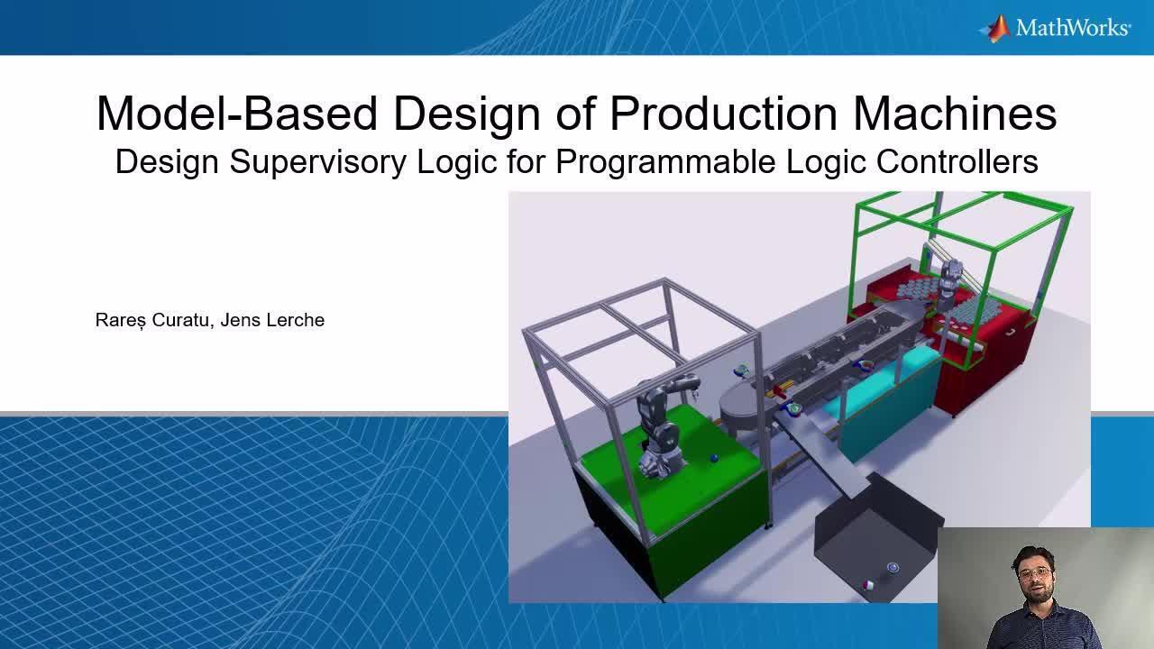
Model-Based Design of Production Machines – Part 2: Design Supervisory Logic for Programmable Logic Controllers

Hello, and welcome to the Model-Based Design of Production Machines webinar series. This is the second part of a four-part series where we're going to talk about the design of supervisory logic for PLCs. My name is Rares Curatu, and I'm an industry manager at MathWorks. Also with me is my colleague Jens Lerche from the application engineering department, who will guide you through the technical part.

Thank you, Rares. My name is Jens Lerche. I am a senior application engineer at The MathWorks here in Germany. And I will guide you through the technical part of today's webinar. Feel free to ask questions in the comments section. And in case you have any questions on your projects-- how MathWorks products can help you there-- feel free to reach out to our sales team, and we will get in contact with you. Thank you.

In this webinar series, we are delighted to share with you a Simulink example that explores the automation of a virtual assembly line. With our powerful tools such as Simulink and the Robotic System Toolbox, we provide you with the ability to simulate and control various components within the assembly line environment. From robotic manipulators to conveyor belts and sensors, you will have the means to coordinate their movement and interactions seamlessly.

Join us as we guide you through the process of designing and implementing advanced control algorithms that optimize your assembly line's performance, enhancing efficiency and productivity. This immersive demonstration offers valuable insight into integrating robotics and automation, enabling you to address real-world assembly line challenges effectively. Thank you for joining us today and for your interest in using MATLAB and Simulink for streamlining the way that you are designing manufacturing equipment.

Here's a system overview of the example that we will be using throughout the webinar series. The model has five components that form the virtual assembly line. The first robot is a Comau Racer T3. This robot picks up the cups and puts them in the shuttles. The second robot is a Mitsubishi RV-4F. The camera sensor in this robot's work cell detects the balls, and then this robot picks up the balls and places each of them in separate cups.

The shuttle track moves four shuttles to robot one, then to robot two, and then to a conveyor belt before returning to robot one. The conveyor belt carries the cups away from the track and into a container. The remaining non-moving model parts comprise the static machine frame, which serves as the base for the assembly. It includes two work cells housing the robots, as well as the base for the central assembly.

In this webinar series, we are starting with modeling and desktop simulation and then moving on to using hardware. These are typical steps when developing machinery using model-based design. After simulating the plant and the desktop environment, designing and simulating the controller, and visualizing the simulations, we will show you the steps that you need to take in order to deploy the control algorithm on a Siemens PLC using Simulink PLC Coder and the SIMATIC Target for Simulink.

This way, the control algorithm that you have been developing in Simulink will be equivalent to the code running on the PLC. To continue the validation and verification of the software on the PLC, We will next deploy the simulation model of the plant on a real time computer using Simulink Real Time in a hardware-in-the-loop configuration. The real-time simulation will then communicate with the PLC through Profinet and also with a 3D visualization of the simulation.

On the screen, you now see the agenda for the entire webinar series and how we plan to break up the content throughout the series. In part one, we have talked about how to import CAD models into MATLAB to then later use them with Simulink. This session was recorded, and you can access it on mathworks.com. Today, in part two, you will see how to design supervisory logic for PLCs using Stateflow.

In part 3, we will talk about how to bring this logic to any PLC or industrial controller. And in part 4, we round up the design process by testing the PLC in a hardware-in-the-loop simulation. During the presentation, if you have any questions, please enter them in the Q&A section. We will gladly answer them at the end of the presentation. Now, I would like to hand it over to Jens for the technical content.

So this is the agenda for the technical part of today's webinar. First, I would like to say a few words about the smart4i demo. In the second point, we will create online trajectories and inverse kinematics for the robots. Then, I will talk about the usage of Stateflow for designing supervisory logic. And in the fourth part, I will walk you through the complete supervisory logic of the smart4i demo and we do a model-in-the-loop simulation.

About the smart4i demo, the smart4i demo is a real life example created by the German company, ITQ. If you do a web search on smart4i, you will find several videos for it. ITQ is an independent service company based in Munich, Germany, and they provided the complete CAD data for this example-- so a big thanks from my side. The demo itself now ships with three toolboxes in 23B-- of course, Simulink 3D Animation, also Robotic System Toolbox, and the Simulink PLC Coder.

There is an option in the Simulink 3D Animation version to include Image Processing and Deep Learning, what requires additional toolboxes, but this is written in the documentation. We don't think that the demo is perfect right now, especially for the automation part that you will see. There are, of course, many other ways you could realize this, but we have plans to further develop it in future releases. And I'm looking forward for the things to come

Create online trajectories and inverse kinematics for robots. Let me start with typical development workflow of autonomous systems. We have various tools for perception, planning, and control. For perception, we offer different sensors, cameras, radar, and LiDAR inside the models. For planning and decision, we have mission and path planning algorithms for navigation and algorithms like obstacle avoidance for manipulation.

In the controls area, of course, we offer feedback controllers, gain schedulers, trajectory control, and supervisory logic. You can also design, model, and analyze your robot platform. And after implementing autonomous algorithms onto your autonomous plant model, you can connect external devices, such as Sensor, or deploy to Target embedded systems. You could do system level design for verification and validation workflow that, combining your system requirements, tests Design Verifier, and so on.

Generate the right trajectory for your application. We ship multiple trajectory generators, such as Trapezoidal Velocity Profile and third and fifth order Polynomial Minimum Jerk for smooth and continuous motion. You can also create constrained time-optimal paths parameterized trajectories that subject to kinematic constraints. That means you can find the fastest possible way to meet each waypoint while velocity and acceleration are constrained.

Let me share a success story of the Hong Kong Applied Science and Technology Research Institute-- ASTRI. ASTRI's challenge was to transition to smart manufacturing to meet customer demand and address rising development and production costs. They needed a more agile and cost-effective approach to build robotic manipulation systems. The solution was the adaptation of model-based systems, engineering with digital twins developed using MATLAB and Simulink.

They created a digital twin for their robotic welding system, embedded with computer vision and machine learning. This approach allows for iterative development and modifications, providing design flexibility and shortening setup time. They also use Synthetic Images and Deep Learning techniques to estimate the position and orientation of the weld piece, along with motion planning algorithms for generating feasible trajectories.

That resulted in a reduction of integration time by 40% and development time by 30%. The model-based systems engineering approach enables resolving functionality issues in the design stage. Thanks to the visualization and testing capabilities of the digital twin, MATLAB and Simulink facilitate collaborative work among engineers, allowing them to work in Parallel, resolve issues, and validate systems as they are built.

So now we are going to see how this is done in the tools. So in the first part of this webinar series, I talked about exporting a CAD files to MATLAB, and-- who have seen the first part might remember that there was the FPX format I used. Or you could use the URDF format-- what is especially beneficial for manipulator export from a CAD tool-- and I will show you why. If you haven't seen the first part, it's available on our website already. So we can put a link in the chat, or you can find it if you watch this part later as well on one page.

So the URDF-- Unified Robot Description Format-- has the advantage that we can also create a rigidBodyTree object in MATLAB. That means we use the import robot command to call the URDF file. And what happened, then, by this command, is that robot one becomes a rigidBodyTree object. And let's check the documentation. RigidBodyTree is a representation of the connectivity of rigid bodies with joints.

Yeah, and with the import format, you can use it in MATLAB. The rigidBodyTree model is made up of rigid bodies as rigid body objects. Each rigid body has a rigid body joint object associated with it that defines how it can move relative to its parent body. That's actually it. So and now, we have our RBT object in the workspace.

And I already, in the first part, gave an overview on the robotics part of the whole smart4i demo. I extracted it a bit to make it more visible in here. So we only have now one robot in here. And we call the scene as shown before, but what we have now is that-- as shown in the slides-- we have the Trapezoidal Velocity Profile trajectory generated for our robot. The waypoints come from our state logic. I will show you later.

Here, we have a little coordinate transformation conversion. And this is the inverse kinematic block. And this is the first time we called the rigidBodyTree object, the robot one we just created. And here, we can select the end tool. And then, it gives the commands back to the individual rigid body parts.

And again, it's calling the rigid body, and we now have to select the body we are addressing in this dedicated block-- same for all the rest of the parts. So now, let's play this. I locked some data from the complete demo-- just for the smaller one-- and I use this replay block that replaced the signals I recorded in the larger model. And now I run it.

And that's the movement we get. And it doesn't pick up cups, of course, because it's really just a submodel just to move the robot. So the URDF format is very handy. It only takes a couple of commands to import it into Simulink 3D animation. And it also helps to control the robot make path planning using the rigidBodyTree object.

Design supervisory logic using Stateflow. What can you do with Stateflow? You can design fault management, supervisory mode logic, or scheduling tasks. With Stateflow, you can represent models as flowcharts, state transition diagrams. This is what we will focus on today. You also have the options to use truth tables and state transition tables.

Before we look into the large state machine of the smart4i demo, I would like to demonstrate you how to create a Stateflow model. Let's begin by choosing a new model. And from the library browser, we pick an empty State chart. We do this in Simulink, but it doesn't have to be in Simulink. Stateflow is also available for MATLAB without the need for a Simulink license.

So now, we are in our chart. We create-- I want to create a simple bang-bang controller. So this is our starting State. Let's call it on. This little arrow shows that the State machine will start in this state. It automatically created this off chart, also these two arrows that will now allow moving from one state to another via the conditions x smaller t0 and X larger equal t0. While we are in an on-state, epsilon equals x. And in the off-state, epsilon equals 0.

There's the simple pan, and it indicates that we have some undefined symbols. We can automatically resolve this by using assumptions. Stateflow does. What's not quite right is that t0 is an input. We want to have this as a local data. We set it to 0. OK, and if we go back, we see we created inputs x and y. We add some sine wave.

This is a simple time of 0.2. Add some scope. Make it two inputs to-- so now, we have a little State machine. Let's do a pacing of the simulation. Just to see it better, make it a real time for 10 seconds.

And here in Stateflow, we can now add some animation. And we can now see-- and we can now see that every time the input is smaller 0, the status of an epsilon is 0. So the output of the chart is 0. And every time it's larger than 0, it's in the on-state, and the input got fed through to the scope directly.

So we are back in the complete model for smart4i example. In part one of the webinar series, I explained the scene creation and configuration part and the animation control part. In this webinar, I explained the robot kinematics. Now, here, we, of course, see it for both robots. And now, let's have a look into this State machine. That's basically the architecture from a top point of view. You can see that the robot one and robot two are more like flowcharts.

With a little exception for a stop state we have here and the shuttles-- these are actually State machines because there are decisions made in which position a shuttle can be. It has a move state, of course. Then, these represent each station in the smart4i production line. Robot one has a station, and there is a park position in between robot two and unload where we have the little slide or conveyor. And then, there is a second park position.

If we have a closer look at the robot, it got initialized as a start. And then, it waits for some sensor signal. This is the above-cup state. Once it's reached its position, it then approaches the cup. It attaches the cup right, raises the cup, moves it above the shuttle. And this is actually where different positions need to be set for picking up the cups and for placing it above the shuttle. Of course, it's always the same position.

And this is mainly a time-controlled flowchart. So after a certain time, it moves on to the next state, detach cup, and then, back home-- quite similar for robot two. And, in between, there are events that trigger back to the shuttle position or the other way around, that the shuttle gives signals back to the robots that they can go on processing. Of course, there are many different options to make such a design-- smarter ones, more time efficient. And I'm sure in the future, there will be different versions of this demo.

So before we finish this webinar, let's do a final run. And just to give you a little idea what is now possible in a sense of debugging a state machine using Stateflow, we add a breakpoint. Let's choose shuttle one. When it goes to-- when it arrives robot one position, set a break point. From the example from before, you know we can also animate the State machine. And let's run it.

So you see, it now pauses the simulation. We can hover over all-- the data's in here-- and have a look at the values, yes, and start to debug our application if needed. And that's it for this part of the webinar series. In the next part, my colleague Mr. Ramirez Garcia will show you how to generate PLC code for any PLC out there using the Simulink PLC Coder. Thanks for your interest.

Thank you, Jens. I really like the demo. This is the end of today's presentation. But before we end today's session, we will be answering your questions. So if you haven't already, please type your questions in the Q&A section. Don't forget to register and attend the next webinars. Taking place every two weeks, we will be going through the steps of designing machinery with model-based design.

If you plan to attend Forum Industria Digitale in Italy, SPS in Germany, or the Precision Fair in the Netherlands this November, we will be happy to meet you there in person and talk about your projects. In the Meanwhile, if you want to take a look at what else industrial automation and machinery engineers are using Matlab and Simulink for, please visit us at mathworks.com/industrial-automation-machinery. Thank you for your attention and for your interest. And now, let's take a look at the Q&A section.