Development of a Signal Processor and Extractor Module for 3D Surveillance Radar

[MUSIC PLAYING]

Hello, everyone. Thanks for joining in. I am Mohit Gaur. I am working as deputy manager in the radar team of Bharat Electronics India. Today, I will be sharing my experience of modeling a signal processor and data extractor module for a 3D surveillance radar.

The agenda for the session will be, we will be discussing about modeling signal processor algorithms and their complexities, the ease of implementation, which was achieved using MATLAB, and quantifying performance during different developmental phases.

I've been working in the fields of radar for the last 12 years. These are the radars I have worked on. I have worked on Rohini, 3DTCR, Revathi, and 3DCAR. Let me begin with a brief overview of the radar system. We all know that radar stands for Radio Detection and Ranging. It works on the principle of electromagnetic wave propagation. RF energy is transmitted, and the energy which is reflected in the form of echoes is received through the front-end receivers, and it is digitized, down-converted for further processing in DSP-- that is, Digital Signal Processor.

DSP performs several functions, such as pre-processing, filtering, clutter cancellation, CFAR-based thresholding. The output in the form of detections is sent to the extractor module, which performs clustering and centroiding. Target reports are then sent to sensor fusion and tracking system, which will generate track outputs. Our focus will be on modeling signal processor and extractor module.

Talking about the challenges that we face, electronic hardware obsolescence is a major challenge being faced today. Legacy languages were used during the earlier days. Their developmental environments have also turned obsolete. The solution to this problem demands both hardware and software upgrades.

Now, to take up any kind of upgrade, we need some form of proof of concept. Now, to model with high fidelity, we would like to validate our development of our model with site-recorded or field-recorded data, actual data. But, for signal processor, that raw IQ-level data is very high-volume data. The recording and handling of that high level of data is another major challenge. The performance evaluation and the nonhomogeneous clutter environment for any signal processor is also one of the major challenge.

As we all know that we are moving towards green energy, wind turbines are here to stay. Wind turbine generators unfortunately generate clutters for 3D radars, as well as other radars. The clutter mitigation for a low-PRF radar is another major challenge. So the requirements for our project were to model signal processor for a 3D radar, to validate it using the actual field data to model the data extractor module, and to realize a kind of test bed, which will be available for proof of concept.

Moving ahead, the algorithmic workflow for the radar signal processor is shown here. Analog IF signal is digitized using an analog-to-digital converter. The signals are then down-converted to the basement for further processing in the DSP. Then it is passed through a filter that is a matched filter that will result in digital pulse-compressed output.

This data is then formatted in the form of radar data cube. The data then passes through MTI pulse cancellers, which is basically used for clutter cancellation. The data now needs to be processed for spectral analysis. FFT technique is used to realize Doppler filter bank. It also performs coherent integration, which results in SNR improvement.

The clutter cancellation is also done based on Doppler filter response. This output is then sent for CFAR processing. The detections are the output of the CFAR module. There are zero velocity filters, which needs to be processed, and the clutter map for detecting the presence of any kind of tangential targets.

Moving ahead, these detections are now sent to the data extractor module, whose algorithmic workflow is shown below. So it includes three major steps. First one is elevation estimation. Then we pass it to the range centroiding and clustering, and then range-azimuth centroiding. The plots are then sent to the tracker module.

Moving ahead, in order to develop this project in a modular manner, we divided this into three major phases, the first one being modeling of main signal processing algorithms. Then, in the next phase, we targeted [INAUDIBLE] validation on the actual field site recorded data. In the last phase, we targeted the modeling and validation of data extractor module.

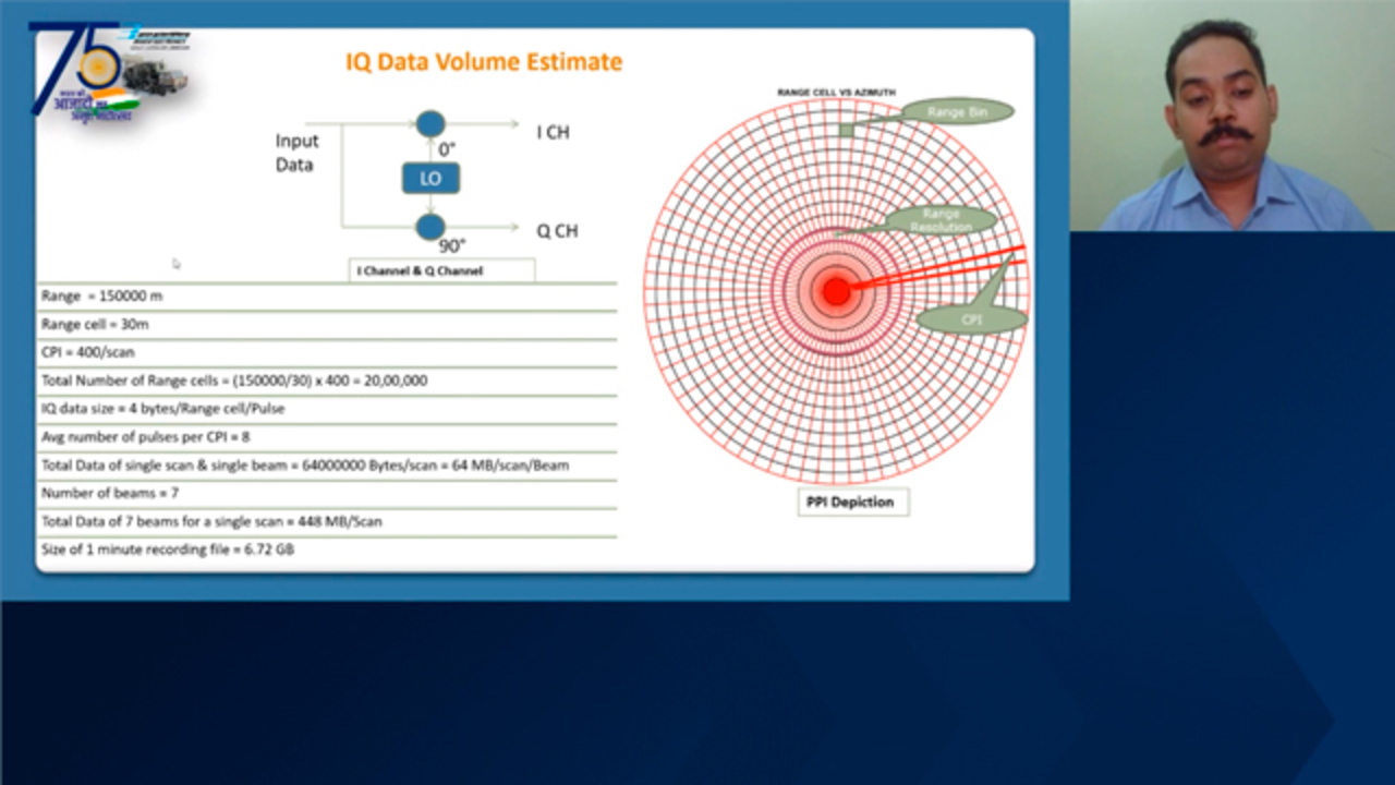
Moving ahead, here, radar PPI display is shown. PPI stands for Plan Position Indicator. It is nothing but a kind of polar plot for better visualization of the radar field of view. The [INAUDIBLE] range is divided into concentric circles, as shown here. The width of these circles is kept equal to the range resolution of period R.

As we are processing multiple pulses at each [INAUDIBLE] position, these red lines are basically showing coherent processing intervals. Between these, whatever pulses we are transmitting, we are integrating them in a coherent fashion. Thus, we can say that the complete range coverage of the radar is divided into a number of arrangements.

Now, since we are using coherent processing for the processing of our signals, coherent means we have to take care of amplitude as well as the phase. For that, we are using both the in-channel and the quadrature channel signals. Now, this is the example that shows how we can estimate the volume of the data in case of the raw data recording.

Let us consider a range of around 150 kilometers. If I keep my range cell dimension to be 30 meters, and the number of CPIs, if I take it as 400 for one scan, then the number of range cells comes out to be around 20 lags. The IQ data, if I am using 2 bytes for I channel and 2 bytes for Q channel, so there will be 4 bytes per range cell per pulse.

And if I am conservatively taking the number of pulses to be equal to 8, then the total data volume comes out to be around 64 megabytes. If the number of beams are also more than 1, which is invariably the case, let us consider 7 beams for our case. So the overall, the size of 1-minute recording file comes out to be around 7 GBs, which is a huge volume to handle. Now, the key takeaway is we can estimate the volume of IQ data using this kind of simple arithmetic.

Moving ahead with the implementation part, digital pulse compression is implemented through matched filtering. We have successfully utilized pulse waveform analyzer app, which is available in the MATLAB, to generate waveform coefficients. The analysis of the effect of the various parameters' variation in the waveform can be readily analyzed using this app. As shown here, I have taken two cases where I have analyzed the transmit pulse width and the effect of windowing during our waveforms.

The figure on the right is basically showing matched filtering procedure. See, here we have generated LFM signal. The figure is showing the transmitted signal. And we have generated ideal target returns, which have been simulated. This last figure is basically showing the pulse compression output, as we can appreciate that the magnitude has increased, and the pulse width has decreased. The main advantage of DPC-- that is, Digital Pulse Compression-- is that it provides better range resolution and a significant improvement in signal-to-noise ratio.

Now, moving ahead, as we know, every radar design starts with certain specifications, such as unambiguous range, range resolution, azimuth resolution, and data accuracies. I have used Radar Designer app to evaluate the effect of variations of certain critical parameters on radar's performance. It helps me to make optimal engineering trade-offs into certain parameters, such as transmit power, transmit peak power, transmit pulse rate, pulse compression gain, et cetera. All these were analyzed.

A high volume of IQ data, which is available to us from the in-service radar, was taken as the input and then arranged in the format of the radar data cube. Here, we are sampling at the rate which is decided by the bandwidth of our waveform. That waveform bandwidth is, in turn, getting decided by the specification of the range resolution. This forms one of the dimensions of the data cube. That dimension is called as fast time dimension.

Using multiple pulses at each antenna being positioned, this provides better SNR improvement because of coherent pulse integration. These multiple pulses are forming the second dimension of the data cube that is known as slow time dimension.

The third dimension is because of the multiple parallel beams which are being used in order to cover the complete elevation span for the radar. And also, it helps in resolving targets in the elevation space. The figure here is showing the plot of received radar echo signal for a single beam in a single dwell or a single CPL.

The next step is the realization of FFT-based Doppler filter bank. There are multiple techniques. Majorly, FFT technique and FIR-based techniques are used. I have used FFT technique. Now, here, if we are using m number of pulses at a particular PRF, this means that we are taking m samples of each range set at a sampling rate which is equal to PRF.

Now, if the signal length is taken to be equal to m, then you can take either m point FFT or next-highest [INAUDIBLE] number, whatever is less. Now, we know that the frequencies which can be represented by the properties of FFT is ranging from half of the sampling rate in the negative side to the half of the sampling rate in the positive side. Now, here, we can realize m number of Doppler filters spanning the frequency from minus 1/2 of PRF to plus 1/2 of PRF. Because we are sampling at the rate of PRF, the central filters will correspond to the zero Doppler.

All the stationary clutter is expected to lie in this zero-velocity filter. These targets, which are moving tangentially to the radar, that is having the radial velocity to be equal to zero, will have a zero Doppler and will fall in zero-velocity filter.

Also, those targets which are moving at the speed other than for which the injected Doppler will become an integral multiple of the PRF, we call them as moving at the blind speeds, because radar is blind to those speeds. They may also fall in [INAUDIBLE] VF or in the edge filters because of the Doppler [INAUDIBLE].

These filters need to be processed with reference to the clutter map. Here, the range Doppler response function, which is available in the MATLAB under Phased Array Toolbox, has been used. That is shown here in this figure. It is basically showing range Doppler map for a single beam and a single dwell data.

Moving ahead, the next step is feeding this data to the CFAR. CFAR stands for Constant False Alarm Rate. Various types of CFAR algorithms are available in the literature. CFAR are used to maintain constant specified probability of false alarm. Since the statistics of clutter, noise, and interference are not known a priori and with certainty, the threshold for the detections needs to adjust itself.

The key advantage for the CFAR detector is that it dynamically adjusts its detection threshold to meet the specified probability of false alarm when compared to the name and VSN detector.

Moving ahead, we started the implementation with a simple CFAR detector that is [INAUDIBLE] CFAR. That is CA CFAR detector. This vehicle is basically best suitable for homogeneous nature of the clutter. Except the zero-velocity filter and the edge filters, all the remaining filters are passed through the CA CFAR detector.

Point to be noted is, magnituding needs to be done before passing the data through the CFAR algorithm. Now, CFAR detector object is also readily available in Phased Array Toolbox. That has been used here. The figure is basically showing the detection map for the single-beam, single-dwell data. Now, the data of all beams, all GPIs, and across scans was fed to this detector object, and detection reports were generated.

Moving ahead, in the next slide, we have plotted the detection reports generated in the PPI format. Here, two beam detections are plotted for ease of representation in different colors. This validation has been done for over 24 scans of data because of the high volume of data. The performance of our model was also compared with the signal processor which is working in the actual radar.

Here, I have also attached the snapshot of the detection map, which is achieved in the actual radar. We could achieve a very close match in the detection reports among the models that we have created in the MATLAB and the one signal processor which is actually working in the radar.

Moving ahead, in the next stage, we have tried to evaluate other CA CFARs, other CFAR algorithms such as GO CA CFAR, that is Greater Of Cell Averaging, and associated, a smaller [INAUDIBLE] CFAR detectors. Here are the results. These results-- basically, these kind of CFAR algorithms are better suited at clutter edges. The results are well within my expectations.

Moving ahead, I will now briefly discuss the modeling of radar data extractor. As I have already discussed in the previous slides, after DSP, the detections are passed through the data extractor module, which will calculate the centroid. This is basically done to reduce the spatial jitter in detections. The output will be smoothened by this extractor module.

So this is basically performing two major functions. One is the centroid-based clustering, as shown in this figure. There are different detections which are available. And these detections are grouped into different clusters. These clusters are formed based on the spatial proximity. The centroid for all these clusters are calculated.

For better appreciation, a figure is shown here. Let us consider these blue dots as detections, and this green star shape is the centroid position. This decision is taken based on their spatial proximity, as well as the strength of the signal which is present.

Now, since in this 3D [INAUDIBLE], we are adding three main dimensions-- range, azimuth, and elevation. So, firstly, we are performing elevation estimation. For this purpose, we are basically using antenna beam pattern.

Here, this data is shown here. This data basically is the calibration data which is received during calibration in the near field testing for the antenna. We have plotted this in MATLAB, and we have got this curve. This basically represents the antenna beam pattern for our radar.

Now, using the MATLAB Curve Fit tool, we have generated the coefficients for the polynomials, which represent the curves for the different sections of this graph. These are then used along with the strength of the detections received for elevation estimation. Here, we can see the different steps in somewhat more detail.

The first step is the receiving detection data from the signal processor module. In this figure, it is showing different ranges along the x dimension, different CPIs along the y dimension. And, along the z dimension, there are the different beams, since we are using parallel multiple stack beams.

Now it can be seen that there are different spreads, that the detection is present in different beams. The elevation is now basically being estimated using the antenna beam pattern. We can see in the next figure that after elevation extraction, the spread in the elevation space has reduced.

The next step is clustering and centroiding in the range dimension. Based on the spatial proximity along the range dimension, the detections are grouped into clusters. Depending upon the relative strength of the detections and antenna beam pattern, the centroids are calculated. Depending on the relative strength of the detections in a cluster, centroids are calculated. This figure shows the range centroided results.

The next step is clustering and centroiding along the range and azimuth. That is in the two dimensions simultaneously. This figure is basically showing different clusters in different colors for better understanding. These will be further smoother after range azimuth centroiding, as shown in the next slide.

After centroiding along the range and azimuth dimension, the output is shown here. The figure on the right basically is showing our model data extractor. And the figure on the left is basically showing actual data extractor which is working in the radar. These figures have been put here for better comparison. The result shows that we could achieve the accuracy of more than 95% during our modeling experiment.

To summarize, we have successfully utilized the features which are available under the Phased Array Toolbox, Radar Toolbox for the different phases of our design and simulation. This has proven to be a very time-saving exercise when compared with the conventional approaches.

With the strong visualization tools and easy-to-use apps which are available with the MATLAB, the testing and performance analysis was done with much ease. We could achieve significant reduction in the development cycle time, as we were able to model with high fidelity. And the best part is, we could achieve the accuracies of more than 95% in our modeling of signal processor and data extractor module.

Finally, I would like to extend my sincere thanks to MathWorks for providing this platform, and special thanks to Mr. Sumit for his excellent technical support. I would also extend my gratitude towards [INAUDIBLE], for their great support and motivation. Last, I would like to special thank Ms. [INAUDIBLE] for her support in modeling data extractor module. Thank you.

[MUSIC PLAYING]