Termination of S-Parameter Networks | Getting Started with S-Parameters, Part 3

Welcome to this third installment in the ongoing MathWorks technical series on the use of RF Toolbox. In this installment, we are going to continue to work with S-parameter Networks. Specifically, we are going to continue to discuss methods for network termination using both standard and arbitrary impedances.

Let's begin by outlining the principal functions that are going to be used today, namely snp2smp, rfinterp1, x and cascadesparams. Again, help for each of these RF Toolbox functions can be found by typing in help and the function name at the Matlab command prompt or typing in the function name in the Help browser.

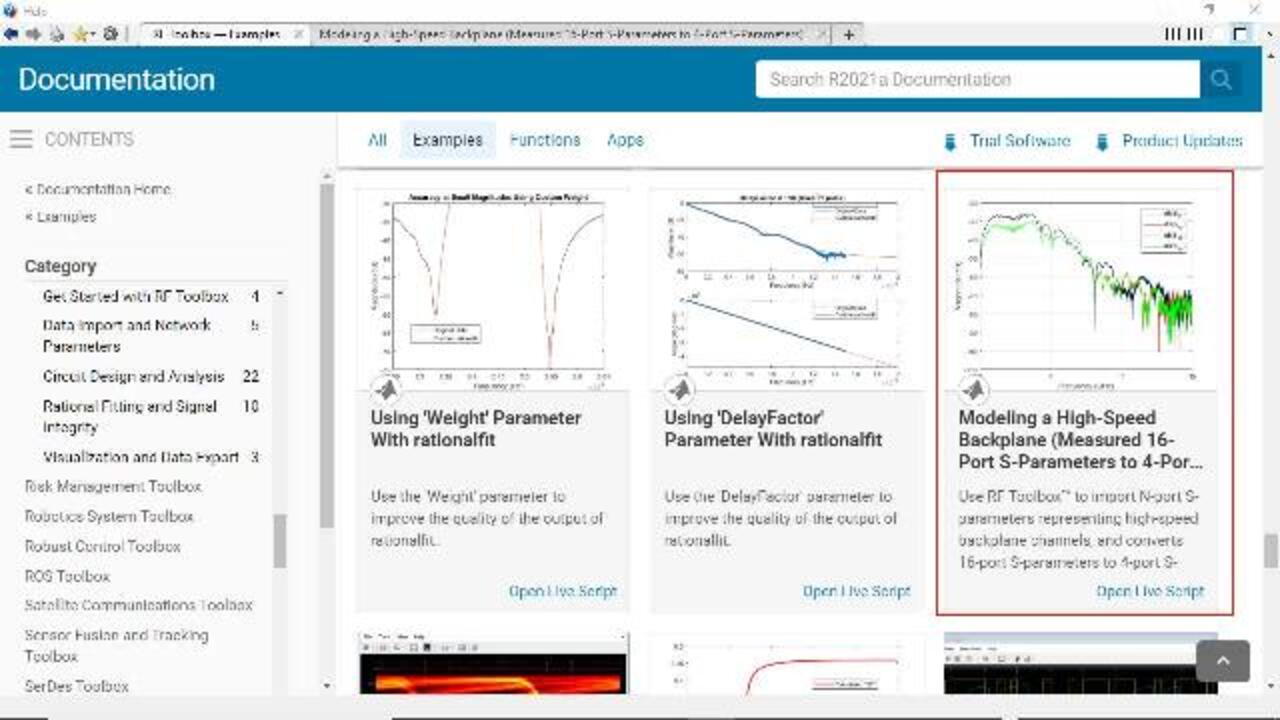
One RF Toolbox product example that I find particularly useful for the use of snp2smp is modeling a high-speed backplane. This example shows the user how to reduce a 16-port network to a four-port network by appropriately terminating 12 of the ports in order to create a single differential channel, useful for signal integrity analysis.

Network terminations can be characterized by single port S-parameter files. These single port networks may use different frequency values from the network being terminated to describe the one-port impedance behavior. If this is the case, it will be necessary to define a common set of frequencies for all elements in the network. When using RF Toolbox you will need to use the rfinterp1 function to interpolate the S-parameters at frequency points in between the original characterization frequencies.

Once the interpolated S-parameters are determined, one can use the cascade sparams function to concatenate arbitrary network parameter files together. The rfinterp1 function is also very useful for converting logarithmically spaced frequency points to linearly spaced frequency points and vise versa. Let us now look at an example where we will use rfinterp1 and cascadesparms. Let us first look at the frequency range of both the three-port network and the one-port load that will be used to terminate the third port of the three-port network.

You will notice that they have both a different number of frequency points as well as frequency values. Since the one-port network has a wider frequency range than the three port, we will use rfinterp1 on the one-port network and interpolate S-parameters over the range of frequencies given for the three-port S-parameter file. Now that both set of S-parameters have a common frequency range, they can be combined to form a single two-port network.

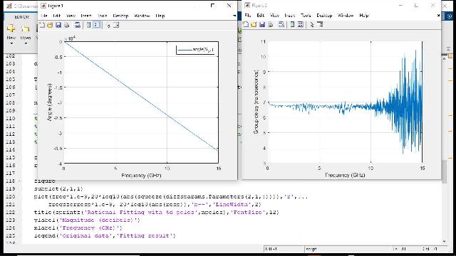
Once this task is completed the reflection response of each of the ports can be plotted and analyzed. Now that both sets of S-parameters have a common frequency range, they can be combined to form a single two-port network. Once this task is completed, the reflection response of each of the ports can be plotted and analyzed.