S-Parameters to Impulse Response | Getting Started with S-Parameters, Part 4

Welcome back to the ongoing MathWorks technical series on the use of RF Toolbox. In this installment, we are going to use RF Toolbox to generate an impulse response for a single-ended channel characterized by S-parameters. We will go over the key functions used for generating the response, as well as documenting the workflow that will be followed. Then, a demonstration will be given that shows the process being used with a backplane S-parameter data set.

Let's begin by outlining the principal functions that are going to be used today. S-parameters, ispassive, makepassive, snp2smp, s2sdd, rational, freqresp, timeresp. Again, help for each of these RF Toolbox functions can be found by typing in "help" and the function name at the MATLAB command prompt, or typing in the function name in the help browser.

One RF Toolbox product example that I find particularly useful for demonstrating this workflow is modeling a high speed backplane. This example shows the user how to convert a single-ended set of S-parameters used to define the frequency response of a channel to a time domain representation by using the RF Toolbox function, rational. In order to convert a channel model or a set of S-parameters into the time domain using RF Toolbox, a structured workflow needs to be adhered. The workflow contains eight unique steps and should be followed each time that you are looking to generate a time domain representation of a backplane or channel model using RF Toolbox.

Let's briefly go through the workflow. First, you will need to import S-parameters into MATLAB. This will be done by using the RF Toolbox function, S-parameters. Once the S-parameters are imported for the backplane or the channel, you will need to check if the S-parameters are passive and, if necessary, enforce passivity. The passivity check helps determine the quality of the S-parameter measurement process and, more specifically, the calibration of the network analyzer used for measuring the backplane. It is likely that the S-parameter data set that you are analyzing has multiple transmission paths, and you are likely interested in analysis of a single differential channel. As such, you will need to isolate a single differential channel from the overall multi-channel single ended S-parameter network.

Before transforming the S-parameters into a time domain representation, it is a good idea to do an informal check of data causality. An informal causality check can be done by visualizing the phase and group delay response of the differential channel. Ascending phase behavior implies a negative group delay or a non-causal response in which a left half plane Laplace domain representation of the data can't be realized. Once you have determined that the S-parameter data is indeed passive and causal, you can then fit a Laplace domain model to the data that can be subsequently used for time domain analysis. The RF Toolbox function used for this process is called rational. The rational fit function has several user-controlled settings which include fitting tolerance and behavior at high frequency.

Once the parameters for the Laplace domain model have been determined, you will then need to compare the frequency response of the model to that of the original data. This can be readily accomplished using the freqresp function from RF Toolbox. Once the frequency response is verified, time domain analysis can then be performed. A time domain response of interest is the impulse response. The method that will be used to generate the impulse response will be to take the time derivative of the unit step response.

One of the advantages of using this process to generate impulse response is that the user can control the size of the time step that will be used subsequently for SI analysis and SerDes lane simulation. This differs from use of the inverse fast Fourier transform methodology where the time step is set by the frequency bandwidth of the S-parameter data file.

Now, let us look at an example that demonstrates this workflow. The example that we will follow will closely resemble the RF Toolbox product example modeling a high speed backplane. We will use a pre-constructed MATLAB script to document and execute the workflow. To begin with, we will use the RF Toolbox S-parameters function to import a 16 port backplane model. Once the data is imported, we will check the passivity of the data and, if necessary, enforce passivity on the data set. It is useful to plot the results of the passivity test. This provides you with a better feel for the passivity test applied. You will notice that for this case, the eigenvalues for the passivity test are between zero and one. If the passivity test were to fail, you would see eigenvalues that lie between zero and negative one.

The next step of the workflow will have us reduce the 16 port multichannel representation and select an individual channel. In this case, the near N channel characterized by ports 1, 2, 15, and 16, will be selected for analysis. Via the snp2smp function, the 16 port single-ended representation is reduced to a four port single-ended equivalent for a single forward channel.

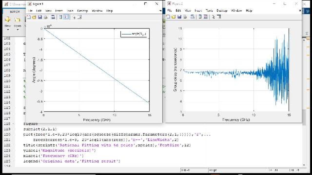
At this point, we will convert the single ended S-parameters into differential mode representation. We will do this by using the s2sdd function and setting the appropriate differential impedance for the calculated differential S-parameters. With the forward channel selected, we will do an informal check on its causality by plotting the phase and group delay response to the transmission path. You will notice that the phase response for the differential forward transmission path is monotonically descending with frequency and that the group delay response is around 6.75 nanoseconds, up to around 10 gigahertz. Above 12 gigahertz, the transmission response is dominated by the noise floor of the measurement device.

As we can see, the behavior of the differential forward channel path passes our informal causality test. Now that the S-parameters have been converted into a differential format, and the test for passivity and causality have been performed, we can generate a model that can be used for time domain analysis. We will use the RF Toolbox function, rational, to generate a rational function fit of the forward channel differential response. Before we execute the function rational, we will adjust some of the function parameters, namely, the tolerance. The tolerance parameter is manually selected to provide a trade off between the frequency domain fit and the model order, or the number of poles found for the rational solution.

With the rational function model now determined, we may want to verify the fate visually. This can be accomplished by plotting the magnitude and phase responses for each of the original data, and the derived rational model. You can see from the plotted responses that there is a good correlation between the model and the original data set.

Now, we can turn our attention to analyzing the time domain response of the calculated model. My personal preference is to always start with calculating the step response of a rational model, and then determine subsequent responses, such as the channel's impulse response. To generate the time response, we first need to define some parameters for the input signal to the channel. Namely, the time step and the number of time points that will be used for calculating the step response. In this case, we are going to use time step that is based off oversampling a 10 gigabit per second data rate by a factor of 64. We will analyze the step response up to just over 100 nanoseconds and validate that the step response has achieved a steady state condition.

With a well-behaved step response, we can use the mathematical relationship that exists between the heavy side Unit Step function and the Dirac Delta function, namely that the Dirac Delta function is the time derivative of the unit step function. In our case, we are going to determine the impulse response by using discrete time differential calculus properties, namely, determining the difference representation of the Unite Step response, and then plotting the result as a function of time. Here, we can see that the resulting impulse response follows an expected behavior.

One thing that I should note is that when you use the rational modeling approach, you can select an arbitrary time step size for the channel's time response. This is an advantage over discrete time methods, where if you want to get around the frequency range limitations that this method imposes, you will need to do a combination of windowing and data padding to be able to generate step sizes conducive to signal integrity analysis.