Electric Motor Control | How to Use Rapid Control Prototyping to Validate Electric Motors and Power Converters, Part 2
From the series: How to Use Rapid Control Prototyping to Validate Electric Motors and Power Converters
Dr. Carlos Villegas, Speedgoat
Learn how to deploy and test a field-oriented control (FOC) algorithm with a PMSM motor using Speedgoat® hardware for rapid control prototyping. Explore how to:
- Transition from desktop simulation to real-time testing by adding and configuring Speedgoat I/O driver blocks for PWM generation and quadrature decoding
- Read phase currents with synchronized analog inputs • Leverage Simulink® dashboard blocks as a graphical user interface to interact with the target computer
- Use the Field Oriented Control Autotuner block from Motor Control Blockset™
- Deploy the algorithm to an FPGA by using HDL Coder™ to increase the achievable sampling frequency
Published: 10 Nov 2021
Let me try to illustrate the main advantages of rapid control prototyping that Diego just mentioned. Let's say that we have a permanent magnet synchronous motor and we want to do speed control under different load conditions. We also have the motor data sheet from the manufacturer. In this case, we are using a permanent magnet synchronous motor with 100 watt rating, seven pole pairs, 24 volts nominal voltage, and a rated speed of 4,300 RPM.
Our final motor drive is still under development. As we will use a standard two level, three-phase inverter topology, we'll start testing with an off-the-shelf inverter from Speedgoat. After checking that the technical specifications of the Speedgoat three-phase inverter are suitable for our test, we'll use rapid control prototyping to make sure that our control strategy and motor can achieve our project's requirements.
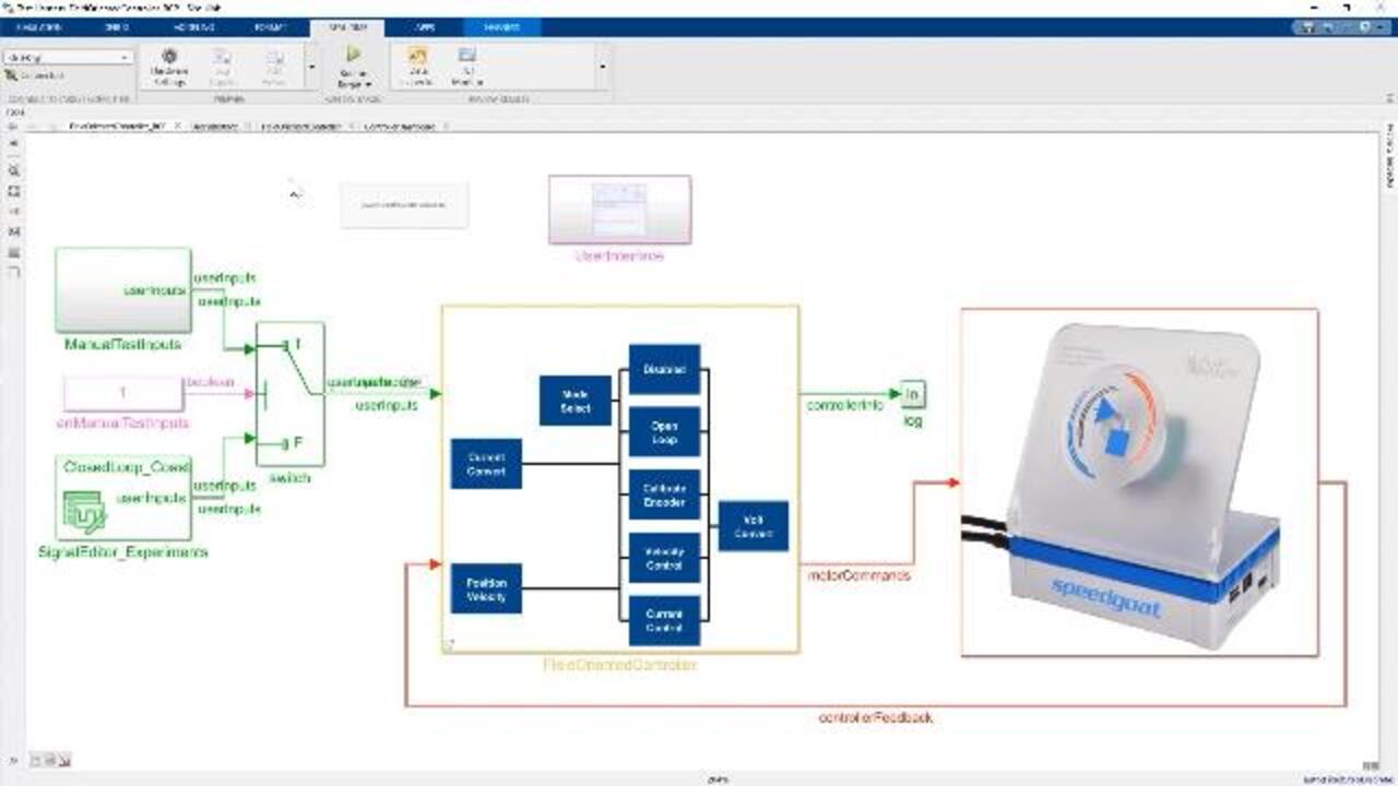
As a motor control approach, we'll be using field oriented control. Let me show it to you within Simulink. Here's our Simulink model for desktop simulation. The two large blocks in the model are the control algorithm on the left hand side, and the plan with a motor, drive, and load on the right hand side.
If we look into the control algorithm, we'll see the field-oriented control blocks, including the typical Park and Clarke transforms, to go from the three-phase coordinate trained to a rotating D Q coordinate train. Once we're happy with the simulation results, we will take the control algorithm that you have just seen and deploy it to the Speedgoat baseline real-time target machine.
This simple diagram summarizes the interfaces between the control on the left, the drive and the electric motor on the right. The control algorithm running in the baseline real-time target machine will obtain the rotation from the quadrature encoder sensor. It will also measure the phase covariance by using analog signals. And finally, it will generate PWM signals to the motor drive in order to control the electric motor. We'll configure all interfaces from Simulink.
A Simulink real-time is jointly developed by MathWorks and Speedgoat, transitioning from desktop simulation to testing could not be easier. Let me show you how it looks in the product. Here we have the blocks for the field-oriented control algorithm. We'll configure the real-time deployment from within Simulink, like the multicore execution, sample time, core size, and the format for each signal.
For example, here we have set 20 kilohertz sample time for the inner current control loop, shown in red. And we also set a slower 1 kilohertz sample time for the speed outer control loop, shown in green.
We configured the FPGA and input-output interfaces from within Simulink. Here, we select an IO397 FPGA. We use a predefined bitstream, built to our needs, that includes an input for encoder measurements. Three PWM channels, an input, and also, general purpose digital I/O.
We are also using analog inputs for the current measurements. Now we also add a PWM generation block from the Speedgoat library. We set the number of channels to three, define the symmetric PWM pattern, set the switching period, add a PWM trigger, and set the sample time to 50 microseconds, or 20 kilohertz frequency.
The three-phase UT cycles will be an input to this block. In a similar way, we can add and configure digital outputs for starting and stopping the motor. It is also easy to instrument. Like here, we can add a switch with a few clicks. We can now connect, deploy, and run the controller to the target, and the motor will start spinning.
We are first just spinning the motor with scalar control. We basically provide three-phasing for the voltages, whose amplitude and frequency will create a rotating magnetic field that will also start rotation of the permanent magnets in the rotor.
As the motor spins, we will be measuring the rotor rotation and three-phase currents using I/O configured with Speedgoat drive blocks, as we create in a similar way as we did before for the PWM generation and digital channels.
We are now commissioning our input and output interfaces with a drive and electric motor. Let us run the model again, and plot the current measurements in real time using Simulation Data Inspector. We then realized that there's a significant bias in the current sensors, as we have not calibrated them.
We can now go to the ADC Transducer Voltage to Current signal conditioning block, and modify the bias vector to remove this offset. As we are running the model, we immediately notice that we have removed the bias of the sensor.
Now that we have removed the bias, let us try spinning the motor again. We measure the current, and we can notice that there is no bias anymore. And as the motor starts spinning, we now have a three-phase current centered around zero. We can also see the rotor speed from the encoder measurements.
We can also log data that we will have on the screen, and compare with different test runs to evaluate performance. We can also compare the performance of different control algorithms or test conditions. We can then see how easy it is to configure real-time execution, connect inputs and outputs, modify parameters, see waveforms, and also log data from Simulink.
But we don't want to just spin the motor, but to test a closed-loop, field-oriented control algorithm. We have already added input and output interfaces using Speedgoat driver blocks to the field-oriented controller, just as we did before with the open-loop example,
We also use a graphical user interface in the Simulink Editor to control the motor and plot the speed. We build, deploy, and run the closed-loop algorithm to the Speedgoat target computer with a few clicks. It is initially in standby state, and we transition to closed-loop state with a switch, enabling the PWM gate drives.
The rotor speed rapidly reaches the speed set point. We adjust speed with the rotating knob. But we could also have done it in other ways, like with the command line, or programmatically. We see some overshoot in the tracking performance of the speed tracking.
Let us tune the control gains using a graphical user interface that we created, and double the P gain, or proportional gain, of the velocity PIT. You can go back to the other user interface and check the performance by adjusting the speed. We should expect for the control performance to be a little bit different than in desktop simulation. Nevertheless, we can always tune the parameters in real time to achieve the desired performance.
Well, we don't really want to spend much time doing manual tuning, especially when we have cascaded control loops and three different PI controllers to adjust. Wouldn't it be excellent to have an automated approach for tuning? We can do this with the FOC Autotuner from Motor Control Blockset.
Unlike embedded platforms, Speedgoat target computers have sufficient processing capacity to handle complex autotuning algorithms during real-time testing. This is a FOC Autotuner block. Here we can set the control requirements, and the autotuner will find all the control parameters automatically.
In this case, we set the control bandwidth and phase margin for the inner control loop and outer control loop. The autotuner will apply perturbations to the speed and current control signals, and use the response to obtain the right control parameters.
Let us build, deploy, and run the field oriented control to the Speedgoat target machine, using the FOC Autotuner. We can see the significant response improvement after the perturbation signals are used for tuning.
With the PI parameter obtained for both control loops, we get a much better performance. The PI parameters are updated within the controller in real time. We can also see the resulting gains with the Simulation Data Inspector, or just using a display during desktop simulation.
With the advent of wideband cap semiconductors, and to reduce noise for electric vehicles, the control bandwidth requirements are increasing from a few kilohertz to at least 10s of kilohertz. Algorithms are also becoming more complex and require faster signal processing capabilities.
We can use FPGAs for those faster control or signal processing needs. One way of implementing our field-oriented control to the FPGA is using an efficient, fixed-point implementation. We can convert the controller we have already to a fixed-point implementation by using the Simulink Fixed-Point Conversion tool.
Nevertheless, we can also stay in Floating Point, thanks to the native Floating Point support in HDL Coder. We can even implement algorithms with large or unknown dynamic ranges, and implement operations that are difficult to design in Floating Point, like the arctangent.
With Floating Point, you are also able to analyze the HDL code generated by your model. It is possible to go to the HDL implementation of any Simulink model that you are interested on so there is full bi-directional traceability.


Seleccione un país/idioma
Seleccione un país/idioma para obtener contenido traducido, si está disponible, y ver eventos y ofertas de productos y servicios locales. Según su ubicación geográfica, recomendamos que seleccione: United States.
También puede seleccionar uno de estos países/idiomas:
América
- América Latina (Español)
- Canada (English)
- United States (English)
Europa
- Belgium (English)
- Denmark (English)
- Deutschland (Deutsch)
- España (Español)
- Finland (English)
- France (Français)
- Ireland (English)
- Italia (Italiano)
- Luxembourg (English)
- Netherlands (English)
- Norway (English)
- Österreich (Deutsch)
- Portugal (English)
- Sweden (English)
- Switzerland
- United Kingdom (English)