Constraint Enforcement for Improved Safety | Data-Driven Control
From the series: Data-Driven Control
Brian Douglas
Learn about the constraints of your system and how you can enforce those constraints so the system does not violate them. In safety-critical applications, constraint enforcement ensures that any control action taken does not result in the system exceeding a safety bound. Constraint enforcement is especially important in learning-based control systems when safety metrics like margins can be difficult to quantize and prove.
Published: 19 Jul 2021
In this video, we're going to talk about constraints or limitations of your system and then show a way to enforce those constraints so that the system doesn't violate them. And this is really important for safety critical applications where you want to ensure that no matter what action is taken, it doesn't result in the system exceeding some safety bound. And this is especially important in learning based control systems where safety metrics like margin can be difficult to quantize and prove. So I hope you stick around for it. I'm Brian, and welcome to a MATLAB Tech Talk.
As the name suggests, constraint enforcement is making sure that your system does not exceed some threshold or bound that you set for it. And perhaps the simplest form of constraint enforcement is a saturation function. This function passes through the input signal unaltered as long as the signal doesn't exceed the upper or lower bound. And if it does, then the signal is capped or saturated at that bound. And in this way, the constraint is enforced because it can never be exceeded. And a possible use case for saturation is for safety or protection in a control system.
For example, you may place it on the output of the controller before that signal goes to the actuator to ensure that you don't attempt to command an actuator beyond what it is capable of or rated for. You can think of the saturation function as a soft stop for the actuator, because it's a software driven limit. Versus a hard stop, which is the physical limit of the actuator. And often it's not a good practice to drive an actuator into its physical hard stop. And so enforcing that constraint in software is preferred.
But in addition to enforcing a constraint on a control action, you may also want to enforce a constraint on the system state as well. It may be unsafe for the system to reach a specific state and therefore you want to protect against that.
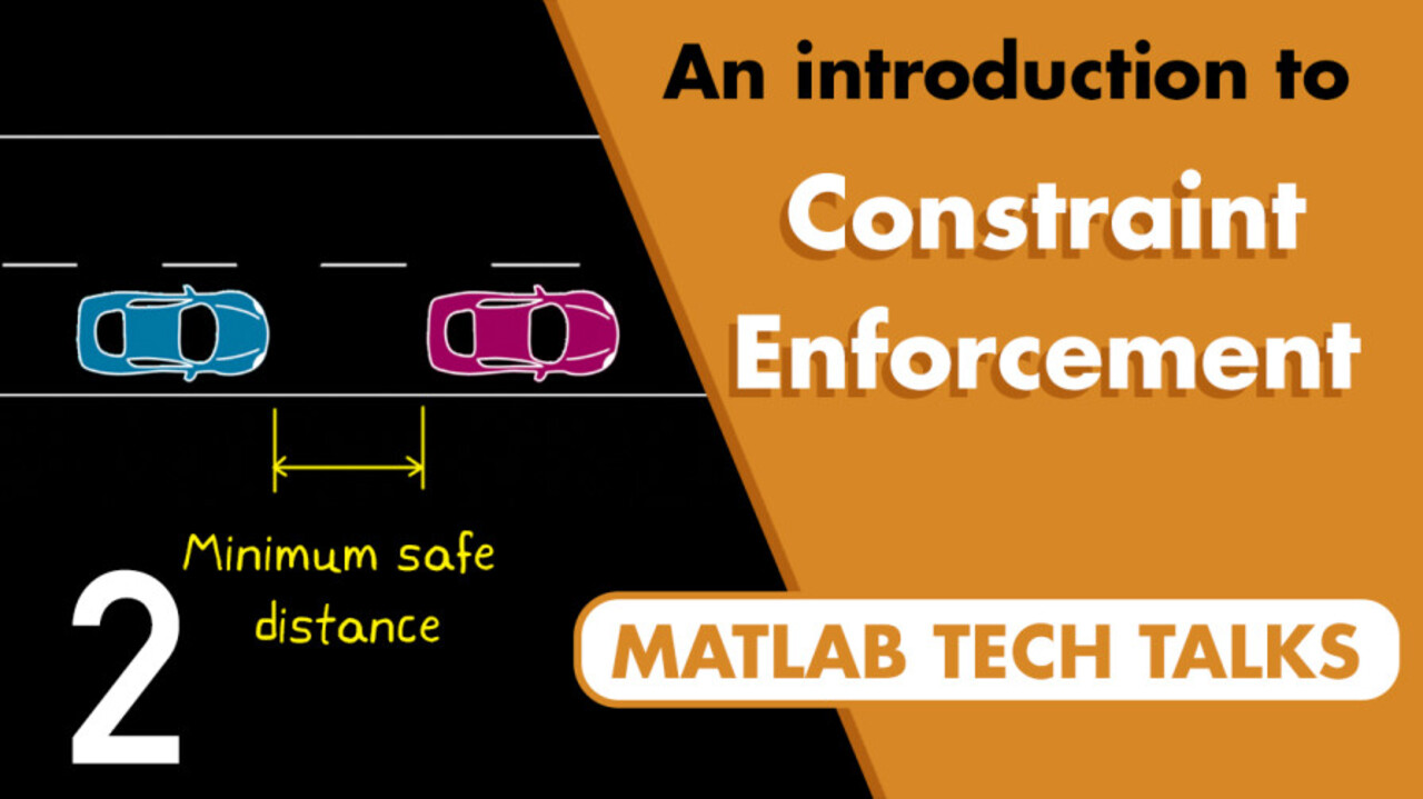
As an example, let's say we used reinforcement learning to develop an adaptive cruise controller. With adaptive cruise control, a desired velocity is commanded by the driver. And as long as there are no obstacles in the way, the controller maintains that constant speed. However, if the vehicle approaches a slower car, then the commanded velocity is obviously too fast and the controller automatically will slow the car down to maintain the set distance to the lead car.
Now, you can imagine that there is some minimum distance to the lead car that is a safety critical state. You don't want this distance to go below some threshold even if the lead car slams on the brakes or does some other maneuver that maybe the learned controller hasn't been trained on. Therefore, just like with the saturation function, we want the output of the controller or the control action to be passed through unaltered if it doesn't cause the distance to the lead car to violate this constraint. However, if the distance constraint is about to be violated, we want to limit the control action such that the constraint is enforced.
And unlike constraining the controller output with saturation, modifying the control action in a way that enforces a constraint on system state isn't quite so straightforward. It's not possible to measure a future state then see that it exceeds the constraint and then somehow go back in time and undo that action. And since we can't do that, we have to use a model to make a prediction of what the state is going to be and then use that prediction to adjust the current control action. This prediction only has to look a single time step into the future. Because like with saturation, we want this function to only step in and modify the input if a constraint violation is just about to occur.
But this is where the time step of the prediction model becomes important. If the time step is too long, then unmodelled dynamics and disturbances will have a larger impact and you won't have as much confidence in the prediction. For example, with adaptive cruise control, this is like trying to predict where the lead car will be after 10 seconds or a minute. At some time scale, there's just no way to have confidence in your prediction since you can't account for the other driver inputs and other disturbances.
However, on the flip side, too short of a time step in the control action necessary to stop the constraint violation in one time step might be too large for the actuators to handle. This is like realizing your car is approaching the minimum following distance 50 miles per hour too fast and only having 10 milliseconds to recognize that and slow down. So there's a trade off here with sample time that is going to be unique to each system.
All right, let's move on. We can create a discrete model in the following state space form. This is saying that the state at the next time step k plus 1 is some combination of the current state plus some combination of the inputs into the system. And we know the current state, because we can measure it. And we know the input u because it's the output from the controller. Therefore, we can predict what the state will be in the next time step. And we want to constrain that state to be less than or equal to some constant.
If this constraint is met, then our function will pass through the input u unaltered. But if the constraint is not met, then we want to modify u in the smallest possible way to meet the constraint. We can write all of that mathematically as minimizing the absolute square of u minus u0, where u0 is the unmodified control action. That's what's coming into this function. And u is the modified one, the one coming out of the function.
But we can take this one step further and combine all of this with a saturation function by adding a lower and upper bound constraint on the control action as well. So here we have two inequalities, the state constraint and the control action bounds and one quadratic cost function. And we can solve this to find an optimal control action u. This is a quadratic programming problem. We're trying to minimize this quadratic function subject to these constraints on the variable.
Now, we could write something ourselves to solve this problem, but there is a quadratic programming solver as part of the optimization toolbox in MATLAB. This minimizes a function of h and f such that these inequalities are met. So now we just need to format our problem into this form, and we can solve for the optimal x, which in our case would be the optimal u or the optimal control action.
Now, with all of that being said, there is actually an easier way to solve this quadratic programming problem and enforce our constraints. And that is with the constraint enforcement block in Simulink. If we open up this block, you'll see a familiar sight. This block minimizes the square of the difference of u and u0 subject to these state constraints and action bounds. Exactly what we just set up in the first half of the video. So let's walk through a simple problem and check out this block in action.
OK. I have here a discrete PID controller that's running at 50 hertz. It's producing a control action that drives this continuous time plant. And if I open up this plant, we can see that it has two states because of the two by two A matrix. And both are outputs of this system since C is the identity matrix. And there's a single input into this system, which is the control action from the PID controller, and it directly affects the first state since the B matrix is 1, 0. And with this feedback system, you can see that I'm trying to control the second state to a reference value of 1.
So that's the setup. Let me run this model, and we'll check out the results. We can see that the output nicely rises up, overshoots 1 a bit, and then comes back down and ultimately settles at 1. Now, for the sake of this video, let's assume that it's a safety concern for this signal to go above 1.1, which it is currently doing.
So to fix this, we could adjust the controller gains so that it doesn't overshoot this much. But this won't necessarily protect us against unknown situations that this system will encounter. And this is where constraint enforcement could come in. Between the controller and the plant, we can place a constraint enforcement block to override the control action when the state is about to cross 1.1. So inside this block, we're going to have a single constraint to enforce, and we want to enforce it at 1.1. And then under block parameters, I'm going to set the sample time to 20 milliseconds to match the rate at which the PID controller runs.
All right, so let's close this, and then we can see these two external ports, fx and gx. They define the model. So let's go create that. In MATLAB, I've created a state space variable g that is identical to the plant that we're using in Simulink except that I've changed the C matrix to only output the second state, since this is the output that we're interested in constraining. Now I'll discretize this with a sample time of 20 milliseconds to get a discrete model.
Again, you may be working with a non-linear plant, which requires a non-linear state space model, but for this example this linear model is sufficient. And this is in the form xk plus 1 equals A times xk plus B times uk with output yk equals C times xk plus D times uk. And we need to fit this model to the form xk plus 1 equals fx plus gx times uk for the constraint enforcement block.
Now again, we're not trying to constrain both systems states but just the single output y. So instead of xk plus 1, we want to model the output in the next time step, which is yk plus 1. And incrementing the output equation by one time step gives us yk plus 1 equals C times the future state plus D times the future input. But as we can see, our D matrix is 0. So this term goes away. And then after doing some substitutions, we're left with yk plus 1 equals C times the quantity A times xk plus B times uk. And in this form, fx equals C times A times xk and gx equals C times B. So those are the values that we need to send into the constraint enforcement block.
And I'll zip through this real fast in Simulink, but basically I'm just setting up the matrix multiplication operations that we just derived. So for fx, I'm looping back the output and multiplying it by C and A. And for gx, it's just C times B. And this is everything we need to constrain the system. And so now I'll run it again and check the scope. We can see that the output approaches 1.1 and then it stops right at it before coming back down and settling at the commanded value. So we can see the constraint was enforced.
And if we look at both the unmodified and modified control actions, we can see that the two are exactly the same everywhere except at about 1.5 seconds where the constraint enforcement block stepped in to lower the control action to constrain the output. But as you can see, it's kind of a rather large negative impulse. And this is what I was talking about with the size of the control action being larger with shorter sample times.
If I had a larger sample time, then the control action would be spread out over a longer time and it wouldn't have to be such a massive impulse. But again, we'd have to contend with a less accurate prediction. So there's trade offs everywhere. But I'm actually happy with this result. So if I wanted to, I could now generate the embedded C or C++ code for this block along with the PID controller and the rest of the control system with Simulink coder. And then the resulting code could then be deployed to my physical hardware to try it out on the real system.
All right. If you want to know all of the details of the constraint enforcement block, you should check out the documentation from its help file. It goes over all of the different parameters that you can tweak and modify. And at the bottom, there are some examples that you can check out as well. There's another PID example, but this one constrains two different states at the same time and a version of that where the constraints are learned. And there's a good video that walks through this PID example that I've linked to in the description if you want to check that out.
And then the last thing I want to mention is that this other example is where you can see how constraint enforcement works in conjunction with reinforcement learning to train an agent to perform adaptive cruise control. In this example, the exploration of the environment is guided or bounded with the constraint enforcement block. Basically, if the agent requests an acceleration command that would cause a violation of the minimum distance between the two cars, then the constraint enforcement block steps in and overrides the acceleration and then the learning process just continues. It's really cool how a simple constraint like this can interact with the complexities of reinforcement learning and produce a safer learning environment.
All right, so that's where I'm going to leave this video. Hopefully you have a better idea of what constraint enforcement is and the different ways that you can use it. As always, I feel the best way to learn a lot of this stuff is to just try it out yourself and see how it works. And the links to several other resources and the MATLAB and Simulink examples that I talked about are in the description below, and I think they're worth checking out.
And if you don't want to miss any future Tech Talk videos, don't forget to subscribe to this channel. And if you want to check out my channel, Control System Lectures, I cover more control theory topics there as well. Thanks for watching, and I'll see you next time.


Seleccione un país/idioma
Seleccione un país/idioma para obtener contenido traducido, si está disponible, y ver eventos y ofertas de productos y servicios locales. Según su ubicación geográfica, recomendamos que seleccione: United States.
También puede seleccionar uno de estos países/idiomas:
América
- América Latina (Español)
- Canada (English)
- United States (English)
Europa
- Belgium (English)
- Denmark (English)
- Deutschland (Deutsch)
- España (Español)
- Finland (English)
- France (Français)
- Ireland (English)
- Italia (Italiano)
- Luxembourg (English)
- Netherlands (English)
- Norway (English)
- Österreich (Deutsch)
- Portugal (English)
- Sweden (English)
- Switzerland
- United Kingdom (English)