Model-Based Design and Prototyping of FPGA/SoC in an Aerospace Application

[AUDIO LOGO]

Hi, everybody, myself Ashish Vijay. I am discipline system chief in aerospace company Collins Aerospace, and I'm here to discuss about model-based design for FPGA development. In this slide, I will discuss why we need to migrate from the manual code to auto-code using model base and what benefit it brings. And we will demonstrate that benefit using a concept and a use case.

With that, I will go to my next slide. So why we need model-based development for FPGA? In the current project, most of the firmware development is done either manually or with minimum support of model-based. And for the applications in aerospace where we need to develop embedded controller, which are algorithm-rich and a lot of process-centric, model-based development is a way forward because this will provide you a unique advantage on manual code.

The objective of developing a framework based on the MATLAB Simulink is that it will help us to do the reusability of the algorithm module as a library block, which we can use to generate auto code. And this will reduce the cost. In some of our applications, we're able to achieve 30% to 40% cost reduction and lead time to 30%.

I'm going to demonstrate how we can do it in a very simple term. It's that, from the requirement database, rather than doing a manual coding, we can do a design model, which is basically in the G-domain with fixed point using MATLAB Simulink SDL-generated blocks. And from there, we can generate SDL code using the proper setting in the environment which will compliance with a lot of modeling guidelines, the U254 guidelines.

And, from there, we can do the logical synthesis based on what type of FPGA family we are using. And from there, we can go and implement inside the FPGA. So in this process, the model will help us in reduction of the time and increasing the robustness of the product.

So, basically, when we develop the model base, we can do rapid development where we no need to worry-- lot of manual, fixed-point calculation and other things which tool can take care. And then we can do a very easy verification and validation using the same test cases that we're going to use in the model base.

This will even help to club the team, where the algorithm team sometimes don't know the fixed point or VHDL coding. And the VHDL team sometimes does not know how to develop that type of algorithm. So it's reduce that gray area and bring the team together to do the rapid development.

So the current method-- what, most of the time, we use is either we don't use the Simulink model, or we use the Simulink model for writing the manual requirement and then doing the hand code or using the Simulink model to generate the test cases out of that and running it for the VHDL. The disadvantage of this method is that the fixed-point algorithm development and verification complexity increases if your algorithms are more complex.

Your requirement to code generation have multilayer and multidomain handshaking, not seamless. In that case, you can have multiple iterations, or there may be chances of the mistake. The closed-loop simulation, the plant model implementation, and the current FPGA development setup is not that easy because it works on this fixed point.

And a lot of time, this control law work and other things-- the algorithm developer understanding the engineering value that convergent and running it in closed loop, developing plant model in the FPGA environment is not that easy.

What method we are proposing is that, rather than using MATLAB or Simulink model only for writing the hand code or test case [INAUDIBLE]-- instead of that, use it as a single source of the truth from requirement spec model to the design model, and generate auto code instead of doing the manual code.

By doing this thing, we can take advantage of modeling loop, testing, generating the RTL. We can do code review, report generation. We can do cosimulation and firmware and loop testing.

The advantage of this method is reducing the time and cost, early validation and verification because we can have modeling loop test cases, and we can use it for the cosimulation. And we can reuse the test cases and plant model throughout the lifecycle. And we do a lot of reusability, scalability, and that will end up in the robustness of the design because we will have less error.

So how the model base can play a role in the DO 254? The three main identify area is-- the first step is doing design by model that can help us in conceptual design, detailed design, and implementation area where we can do our design itself by model and generate the code out of that.

The second step is verification area, where we can use the cosimulation and can do a lot of verification-- early verification or validation-- bridging modeling loop and cosimulation. The third step is that we can use it for firmware and loop testing and a lot of other area where we have to do the physical verification.

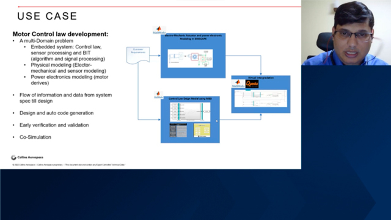
So I will present this framework using a simple use case, which is a motor-control law development. Why I'm using a motor-control law development is because it's a multidomain problem where you have to develop a control law, which mostly go inside the embedded system where you have to do the sensor processing, built-in test. It's a lot of algorithm and signal processing come and play role.

And then physical modeling-- because when you develop control law, you develop for some plant or some actuator, and you have to mimic that plant model using physical modeling, like electromechanical or sensor modeling. And then our electronics modeling, where you have to do motor drive.

So, basically, in this example, we can have customer requirement which can be used for development of the plant model, power electronics side. And same requirement can be used to develop the control law for the same plant model. And, finally, we can do the virtual integration using MATLAB for modeling loop and MATLAB plus [INAUDIBLE] for cosimulation.

So I will go to the next slide from this. To take a very simple example, I'm taking a DC bus motor, which takes the voltage at an input and gives speed as the output. It's a simple, single-input, single-output plant model, just to demonstrate the use case, rather than adding complexity in the use case, and a simple PI controller with a saturater block in S-domain.

This can be the starting of your development on the system level and can become a spec model. This model will be tuned for a given requirement. And once you are able to meet that requirement, you can freeze the architecture, topology, and gains.

So I am able-- I'm showing it by using a yellow line, which is a speed command, and the blue line, which is a speed feedback-- a classical step response, where you can see the motor is trying to catch with the speed command with a certain overshoot.

And if this requirement or this performance-- if this performance is as per the requirement, then we can go ahead and do our design model implementation using same MATLAB, where we can use the fixed-point G-domain or floating-point G-domain. So in this example, I brought the first S-domain model, which we already discussed with the plant model.

The second model, which is in the green color in the middle one, is a fixed-point FPGA model using the Simulink fixed-point block library which can generate auto code for VHDL. And the third one, the last, is the DSP model which, again, is a G-domain but in the floating point.

And I created instance of the same plant model three times so we can compare apple-to-apple results. After running the simulation, if you will see, for the green color, which is the speed command-- same input-- you can see the red color is the floating point DSP model. The blue color is the FPGA model, and the yellow color is the spec model, which is in S-domain.

They all are very near to each other but not similar. The reason behind that is S-domain model is in continuous domain, and G-domain model in the fixed-step size. So sampling error and then the quantization error for the fixed step and the floating point gives some variation, which is acceptable.

If you see the classical result for a step response, like the rise time, transient time, settling time, overshoot, undershoot, or peak time, you will able to see there are some small changes. But if the fixed-point model is it still meeting the requirement and within the tolerance, which, in some of the cases, either second decimal or third decimal-- if is acceptable to us, we can freeze this model and then use it for the code generation.

Now, in this, the advantage of using MATLAB is that you can run a lot of MATLAB script in build function to do the postprocessing of the step response or FFTL-- that type of analysis. It sometimes is not easily available in FPGA development environment.

And you can convert the fixed point to the floating point or engineering number, so everybody, from system team to the firmware team, can easily understand them. Now, I will go to the next slide.

Once your VHDL is generated, you can synthesize it. And now you can bring it back in the MATLAB using SDL cosimulation, where your code will run inside the [INAUDIBLE], you can mimic the FPGA platform or the FPGA device you are intending to use, and you can check the latency, timing constraint, routing, all these things.

HDL cosimulation provides a lot of advantages. It provides you a design verification and validation where you can do your verification against the requirement to check your implementation is correct. It validates your drive requirement, such as sample time, discretization, and fixed-point size because, in the closed loop, sometimes fixed-point size can bring the unstability or some oscillation.

So in the one platform, integrated manner, you can check all these things, not only the functional and performance, even robustness. In the second step is help you in the virtual integration. Within the multidomain-- this type of application-- you can do a proper interface. You can check the algorithm correctness, dynamics of the system, and all these things. So cosimulation can be a very powerful tool for this type of application.

Now, I will show you can use cosimulation by two methods-- the method one, where, when you do the cosimulation process in the MATLAB Simulink, it automatically generates a test harness for you where it will bring the [INAUDIBLE] using a S-function. And it will take the same input, what you are providing to the fixed-point G-domain model which you use to generate the code.

And then it will compare output of these two models, but it will not connect it with the plant model and will not do the closed loop. This type of method can be very good when you have an open-loop type of system, and you don't want to do the closed-loop testing.

In this case, when we run it, you can see the cosimulation results in the top and the difference between the cosimul-- and the second one is the G-domain model, which we use to generate the code. And the error between these two model is 0. It should be because they both are running in the same sample time at the same fixed point automatic, so there is no problem in this.

And we can see that it's proving that you are generated code. You will able to behave in the same manner that your model is behaving in the model environment.

Now, you can see your result in [INAUDIBLE], also, where you can see the speed command and the speed reference, a step command, and other thing, and clock. And all of the things, also, you are easily can see, and you can connect them.

You can do the other method, as well. In this method, you no need to use the auto-generated test harness. You can use the cosimulation S function, and you connect it with the same plant model. So in this example, again, the top one is the S domain model. It's connected with the plant model.

The second one, the green one, the middle one is the FPGA model, which is a G-domain fixed-point model, which we'll use to generate the code and call the cosimulation. And it's calling the same plant model, different instant.

And then the last one is the cosimulation model in S function form, again connected with the same plant model instance. And we are using the same sampling rate, same input to all three. But the feedback is coming from respective plant model.

And then we are collecting the data in [INAUDIBLE], the speed command and then the speed feedback from the S-domain model, speed feedback from the fixed-point G-domain model, and speed feedback from the cosimulation from [INAUDIBLE] VHDL code, which we generated autocode.

Now, if you see the result, the green color is the speed command. The yellow color is the S-domain speed feedback.

And you are only able to see the red color, which is, of course cosimulates any speed feedback because the blue color and red color is superimposed on each other, which it should be because they both are running on the same clock, same fixed-point site. And they are running against the same plant model, then they shall give the same result to us.

Same result you can see in the cosimulation. And you can extract that data of the cosimulation. You can extract the data of the MATLAB Simulink models and can do the postprocessing. And you can see, the results are coming pretty similar-- sorry. They are not pretty similar. They are exactly same, which supposed to be.

With this, I completed my presentation. And I am open for any questions regarding this presentation.

[AUDIO LOGO]