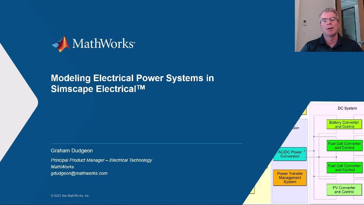
Modeling Electrical Power Systems in Simscape Electrical
Overview
In this webinar, MathWorks will demonstrate modeling and simulation of electrical power systems using Simscape Electrical™. The presentation is developed for students and educators looking to understand the capabilities of Simscape Electrical for the learning and teaching environment.
Highlights
Through a worked example of a mixed AC/DC microgrid system with traditional rotating machinery, AC/DC power conversion, battery, renewable energy and fuel cells, topics that will be covered include:
- Introduction to Simscape Electrical
- Selecting appropriate model fidelity for a given engineering task
- Animating simulation results to support visualization of system behavior
- Ensuring behavioral consistency across a range of model fidelities
- Preparing models for real-time simulation and deployment as digital twins
About the Presenter
Graham Dudgeon
Principal Product Manager – Electrical Technology
Graham Dudgeon is principal product manager for electrical technology at MathWorks. Over the last two decades Graham has supported several industries in the electrical technology area, including aerospace, marine, automotive, industrial automation, medical devices, and power and utilities, with an emphasis on system modeling and simulation, control design, real-time simulation, machine learning, and data analytics. Prior to joining MathWorks, Graham was Senior Research Fellow at the Rolls-Royce University Technology Centre in Electrical Power Systems at the University of Strathclyde in Scotland, UK.
Recorded: 25 Jan 2023
Hello, everyone. Welcome to this webinar on modeling electrical power systems in Simscape Electrical. My name is Graham Dudgeon. It's a great pleasure talking with you today.
Here's the agenda for today. First of all, we'll start by accessing content for this webinar on File Exchange so you're able to download everything that I'll be showing you today, and more besides. And you can use those files, models, and scripts at your own leisure.
The key themes that we're talking about today-- the topics includes the selection of simulation solvers, how to select appropriate model fidelity for a given engineering task, how we can use animation to complement the visualization of results and other engineering results we're looking at to gain more insight into the operation of the systems, and help build our confidence that we're seeing expected behavior. And perhaps more importantly, when we're not seeing expected behavior, how that can guide us to what the problem might be.
We'll also look at how we can ensure behavioral consistency across a range of model fidelities. We do that primarily by inspecting results from simulation to simulation, and basically have that audit trail of simulation models and being able to compare and contrast as we go depending on the range of model fidelity. Then, we'll look at preparing models for real-time simulation and deployment as digital twins before ending with a summary.
So let me just close down that presentation slide, and now we are in MATLAB. But before we get started, let me bring up a web browser. So in MathWorks File Exchange-- so in Google, you can type File Exchange. It will take you to MathWorks File Exchange, and what you want to do is search for our hybrid AC/DC microgrid with PV battery and fuel cells.
And when you're in here-- see there's a link to GitHub? So select that, and this entry here that I'm hovering over-- modeling electrical power systems webinar, dot, zip. That contains all the files that we're looking at today. So then, we'll extract it, and then you'll be set up to do everything that I'm doing today and more besides.
I'll just close this window down. Bear with me a second. So when you extract that zip file, you will have four directories-- solvers for power system simulation from microseconds to years, micro-grid, and model deployment, and real-time simulation.
Now, because we're time-constrained today, as I'm working through these directories, I'll be skipping things as I go, but you can always go back and take more of a look yourself when you download these files. We may not have much time to talk about model deployment and real-time simulation today. If we don't, take a look at that at your leisure.
So let's, first of all, go into directory one, solvers for power system simulation. Now, each of those directories has a MATLAB live script-- a .mlx file. So double-click on the MLX file, and every step is listed here. So we'll start working through it, and I'll make appropriate observations-- I'll run models as appropriate. But as I said before, I may be skipping things in the interest of time.
So at the highest level, when we have an RMS-type simulation-- say a root-mean-square simulation-- the solver options that are available to us are fixed step and variable step. And when we look at the solver choice, typically, for RMS-type simulation, the variable step solvers will give you a more accurate result. Now, the reason for that is the available step solvers are monitoring the delta of the responses.
And when you've got fast acting dynamics, the variable step solver will reduce the time step in order to capture those accurately. But when you start moving more to a steady state or a slowly moving operating condition, the variable step solvers will take larger time steps. So with RMS-type simulations, typically, variable step is more accurate and can lead to decreased simulation times because they're able to take large time steps in those periods where the system is slowly moving.
And the example I'm showing here is field voltage response following a load shed for a basic system I was looking at. You may notice the field voltage goes below zero. It goes negative. That's because I didn't limit it appropriately here, but the main point I want to raise here is I've got two simulations which are different.
I've got a fixed step solver with a 1 millisecond time step, and a variable step solver which is adjusting its time step according to the dynamics, and you can see that they're different. In this particular case, the variable step solver will be your golden reference. That will be the most accurate result because it is modifying its time step resolution. And in this figure, we're looking at here, the red line is the size of the time steps that are being taken. So as we have the fast acting dynamics, the variable step solver is reducing that time step.
Now, variable step solvers, as I said, for RMS simulations can be very effective and can serve as a golden reference. Perhaps you're simulating a system, and you're not 100% sure what the response should be. Variable step solvers could be a good choice there to get that accuracy.
However, for power systems and power electronics, variable step solvers typically are not the norm, and one of the reasons is when we're looking at electromagnetic transient simulation, you have periodic waveforms, and the voltage and current are periodic. And so we need to select time steps which can capture those periodic waveforms to a suitable level of detail.
And the figure I'm showing you here, I've got three examples where I've taken 10 samples, 50 samples, and 100 samples of one periodic waveform. You can see the more samples you have, the more accurate the waveform has been captured. And typically, 10 samples per period is inadequate.
I mean, you can see here that you've not really captured that periodic waveform very well, but the other downside as well with a lower number of samples is you're actually phase shifting that waveform. You can see how if you just picture that as phase shifted across-- and that as well is a detriment for AC system operation. So as a rule of thumb, when we're looking at waveforms like this, at least 50 time steps per period is what you're looking for on your fixed step solvers.
When we're working with Simscape and Simulink, we have the notion of local and global solvers. And let me just highlight this section and then press one section. You can see the MATLAB live script-- I've got code embedded.
And so when I run this, it will initialize parameters and open up this model that we're going to be looking at. And this is a simple example. We've got a simple electrical system modeled in Simscape.
This is the component you can see with the blue lines here. That's Simscape for those of you who may not be familiar with Simscape. Simple DC source voltage source, a switch, and a resistor-- very basic.
And what I'm doing with this switch is I'm driving it through pulse width modulation. But I've got two examples of this model-- one where Simscape is using the Simulink global solver and one where Simscape is using the Simscape local solver. So what's the difference? Well, the Simulink global solver is the solver setting that's set for the entire simulation.
If I right-click and select model configuration parameters, and go to Solver-- we can select variable step and fixed step. I'm just staying on variable step for this example. I've selected that solver as auto.
I'm going to let Simulink decide which solver to use, and Simulink does this by parsing the model and determining what a suitable solver selection is, but you also can manually choose your solvers as well. There's a range of different solvers depending on your needs. I'm leaving it as auto.
So that's the Simulink global solver. Now, the Simscape local solver-- every Simscape model has a solver configuration connected to this block here. Let me double-click on this. I've selected use local solver here, and I've set a time step-- ts.
Now, what's going to happen here is Simscape will use its own internal solver, fixed step, and it presents its results to Simulink as a discrete model. If, on the other hand, we do not select use local solver-- so in the model on the left here, I've not selected use local solver-- the Simscape model will use the Simulink global solver to update, and there are differences.
So let me simulate this first, and then I'll talk through what the differences are. The first thing is you see I've annotated what the signals are. So cont is continuous. FIM is actually Fixed-In-Major-- Fixed-In-Minor time step. It's a continuous signal.
But D-- whenever you see a D, it's like a discrete. And as you can see, when I'm using the local solver, that voltage measurement signal is presented to Simulink as a discrete signal. However, the pulse width modulation in both cases is using the continuous solver which, in this case, it's variable step discrete, so it's adjusting its time steps.
The reason that Simulink selected this is because of the PWM. And we have crossing points between the modulation and the carrier wave, and whenever we have these crossing points, we call those zero crossings. And Simulink, with a variable step, it can detect very precisely those crossing points.
So both PWM generators are the same, and I can verify that by looking at the upper scope here-- just double-click on it. And you can see the pulse train here, where we get to very narrow pulses in the middle of the simulation, and then they expand out-- the typical type of pulse train we see with PWM. So they are both the same. They both capture the resolution very well.
The difference comes in the physical attributes. So in this case, I'm measuring voltage. So I double-click on the voltage scope-- the upper is the voltage measurement from the local solver simulation.
I've set the time step to be 50 microseconds, so my resolution-- my pulse resolution cannot be any less than 50 microseconds. And so you can see that the voltage measurement, despite the fact we're generating a PWM signal that's of high resolution, the physical simulation is constrained by that time step.
So one way that we can get more resolution is to change our time step. So if I go to MATLAB-- so ts is-- this sample time is currently 50 microseconds. If I set that to 1 microsecond and rerun this simulation, a much smaller time step now, so I'll take more time to simulate.
But when I compare, you can see now that it's more accurate with 1 microsecond. So you may be wondering, why would we ever choose local solver? Well, this is a basic example I've just showed you, and it doesn't show the true nature of the simulation attributes and the modeling attributes that we need to consider when we're going to larger scale systems.
And local solver for larger scale is typically more efficient at simulating. And as power engineers and power electronic engineers, we typically like to see fixed-step simulations. There are times, of course, when variable step is perfectly adequate in what we might be looking at, but we do tend to like fixed-step solvers.
But for larger scale, the main point is it's typically a more efficient simulation. I would also say that the cost of the solvers is determined as well. It's like a fixed computational cost for fixed step. With variable step, sometimes the simulations can slow down if there's a very fast acting dynamic and the variable step solver trying to figure out what's going on.
So sometimes you don't have that consistency of computational speed, so fixed step does offer that-- local solver does offer that. And so it's a trade-off. What time step are you going to select for your simulation in order to capture the accuracy you're looking for? But certainly, the ability to detect zero crossing and can be very beneficial.
I'll go back to the live script, and let me just close down this model. So I'm just scrolling through elements that we've already discussed, and in the interest of time, we're going to skip. I've also put a section in here that gives more detail on power electronic switching. And when you are looking for that very high accuracy of the PWM transitions-- the resolution of those pulses, you certainly do want to use the solvers which include the 0 crossing.
And I'm not going to run these models here, but if you go through this in your own time, I've put an example together, which highlights the value of being able to do zero-crossing, and some of the considerations that you need to think about regardless of-- just from a consideration of being a power engineer, and thinking about what information you need when you're doing a simulation, and how the solver can map against that. So I've put more information in here.
And as I said, you can work through these at your leisure. And with the zero-crossing solvers, you tend to get very high resolution on your PWM. But for larger systems and for other types of systems simulation, you may decide to give that up in favor of fixed time step local solvers.
So I'll just slowly move this, but I do want to stop here at the modular multilevel converter. And I want to stop here because I want to talk about two things-- solver profilers and also harmonic analysis, which is invaluable when we are looking at power converter simulation in order to satisfy ourselves that we're seeing what we expect and also to help guide us towards any potential issues that may be in that simulation model. So let me just run this section here.
So what I'm doing is I'm bringing up a modular multilevel converter, which I modeled with full switching effects. And I'm programmatically running the solver profiler with this line of code here, and it's going to show the results on the right-hand side. And so a couple of things to note here.
With the solver profiler, it can show you how many steps were taken during the simulation. It shows you the time, how many zero-crossings occur, and a number of other metrics which can help you satisfy yourself that the solver is behaving exactly as it should behave. So we're using a zero-crossing solver in this case.
And one of the important things with power converters is making sure we have the correct harmonics, and so I'm just going to show you how to run that analysis now. So I've already ran the simulation. You double-click on the power grid, go to Tools, then FFT Analysis.
And this is going to bring up the FFT analyzer, and we'll do a harmonic analysis of the voltage. I'll go to voltage, and I want to look at harmonic order, so select frequency axis as harmonic order. Maybe go up to 5,000 hertz as our maximum frequency for analysis, and we compute FFT.
So you can see things are looking a little bit messy here, but we have our first significant harmonic sidebanded around the 10th harmonic which, for this particular example, is what we expect to see. We have two cells on the modular multilevel converter per half arm, and we have a carrier frequency that's five times our base frequency. So if you multiply the cells-- 2-- by the carrier frequency harmonic based on-- relative to base frequency-- 2 times 5-- 10th harmonic.
And so we can satisfy ourselves that this looks fine. Visually, it looks fine. Harmonics look OK. Let's step up the carrier frequency to be something a little bit more reasonable. Typically, carrier frequencies are much higher than the base frequency.
So we'll run this section with a carrier frequency of-- increased to 6,000 hertz. Run that section, and then we'll do the same thing. We'll look at the FFT.
[COUGHS]
Excuse me. Because we've multiplied our carrier frequency-- we've increased that-- we expect to see those first significant harmonics move up. And so let's just bring this over.
I want to select Vabc in this case. See, it's-- the FFT analyzer is on the first period here. I can change the start time, say, to 0.02. It moves it up. So you can select that region you're looking at.
Harmonic order-- I'll say 10,000 hertz and compute FFT. So you can see, we are sidebanded around the 100th harmonic, and this looks very clean. And so this is one of the key points when we are looking to verify-- or build our confidence we're seeing expected behavior.
Power converters-- the architecture and the switching frequency of the PWM strategy that we're using will result in a very specific harmonic signature, and so we expect to see that harmonic signature. In this case, we expect to see the 100th harmonic being the first significant harmonic suitably sidebanded, and we're seeing that.
So let's now break something. So let me just go into this model. I'm going to go to positive arm A. Go into the cell-- just double-click on the switches. And I've set this up so I can actually fault a control signal by changing gain to 0.
So I've basically broken the control signal to switch two on cell one. And we can run this simulation, and reload the voltage, and compute FFT. And you can now see that the FFT is changed.
We now have a harmonic at the 100th harmonic, which we did not have before. So visually, when we're looking at these plots-- or just the time series data, it may not expose the problem. We can-- despite our own experience and expertise, you may not see things on the time series plots, so you really do need to supplement with these additional analyses to give you that additional insight.
Let's just go back to normal operation. Run this again. And then we'll just run the FFT again, so just reselect-- recalculate. And I just zoom in.
You see that's now gone. It should be there. And so when you're seeing harmonics that you shouldn't be seeing, it indicates that there's a problem. I'll just close this down.
[WINDOWS CHIME]
There's an example with more switches as well you may want to take a look at your leisure. That's an interesting one as well. If you decide to break this, you'll see some more interesting harmonic effects going on.
But the final simulation I want to talk about in this section is a phasor simulation. Now, in Simscape, we call it frequency and time and formulation. So we've looked at point on wave simulation, so EMT-- ElectroMagnetic Transit-- this point on wave-- where you need that time step to be small enough to capture that waveform.
But another mode that we can use is phasor, where we instead represent the electrical quantities as phasor magnitude and angle. And when we do that, we can take larger time steps. We don't need to take such small time steps anymore, so we can increase the time step, run faster simulations.
But we need to appreciate that we lose information, and the information we lose is point on wave. So I have an example here-- EMT and phasor. And if you run that, you can do a comparison between the EMT simulation. In this case, you can see the voltage waveform, which is characterized quite well because we have a very small time step.
And then on the frequency and time simulation-- or phasor simulation-- you can see the magnitude, and we can also look at the angle. Let's actually run this. So I'll just run section and just show you this example.
So same system, but the solver configuration for the phasor representation-- see, equation formulation offset is frequency and time. And I've got a sample time of 1e minus 2. And for the EMT, I've selected time as the equation formulation-- a sample time of 1e minus 4. More of this when we get to the system, because I've got a comparison where I'm-- where I have the full microgrid, one with time formulation on the AC side, one with frequency and time, and we're going to compare and contrast later on in this webinar.
So let me close this down, and we'll move on to the next section. Section 2, from microseconds to years. So look for the MATLAB live script. Open that up.
Now, the intent of this section is to talk about the time scales of interest, and different engineers need different time scales when they're doing their engineering tasks-- certainly, parallel electronic engineers who wanted to see the harmonics and the effect of switching.
Do you need to model the switching? Do you need to have a time step that's appropriate-- potentially, the microsecond level in order to see the detail that they need. But you can start making choices on model fidelity and depending on the engineering task.
So let's go through this. And the system we're using is actually a PV array. And we're going to start with a detailed parallel electronic switching system, and we're going to work backwards.
So we're going to strip the detail away and extend the time scales, and I'll talk about why we're doing that, and what that leads to, and how that benefits different engineering tasks. So let's open the system solar MPPT DC microsecond. So I'll just open that up and I'll take a quick look.
We'll be revisiting the PV array later when we're looking at verifying this operation. But for now, what we have is a certain solar panel, and it's connected to an ideal system connection. We're using a maximum power point tracking algorithm. So this is based on perturb and observe, where we are adjusting duty cycle.
And it's looking at the power gradient, and it's attempting to move the power gradient to 0, with the theory being that when you move to the 0 power gradient, you're at maximum power. So we'll adjust duty cycle appropriately and take as much power as it can from the panel through to the ideal system.
So let's just run this with the microgrid-- sorry, the microsecond resolution. I'll just bring up the data inspector as we're doing this. So this is Simulation Data Inspector, where we're able to log signals and view them.
And we keep track of the runs, so this is very valuable as we're stepping through different resolutions to be able to do this and to compare and contrast simulation runs, which we're going to do here actually with our models. So you can see, it's a relatively slow simulation, but we are at microsecond resolution, and we're seeing a ramp in the cell current.
And I've just done a simple profile for this particular example. So we'll just let that run to completion. And while we're doing that, the next model I want to show is a millisecond model.
So let me show you some details in this model. If I go to the boost converter that we're using, it's a fairly detailed switching model in this case, which I'm driving with a PWM generator. And the PWM generator is a 50 kilohertz timer, so I'm down at the microsecond level.
Now, say I'm the control designer, and I want to design the algorithm-- the MPPT algorithm. I don't necessarily want to wait these long periods of time with the detailed simulation in order to get design feedback for me to modify that design. Instead, I would typically want to operate a millisecond level where I'm not considering the detailed electronic switching, and so operate with a different fidelity of model.
And I'll just bring this through. See, on the phase of it, it's the same, except now, the boost converter is an average value converter, and we're not generating PWM signals because we have no switches to turn on and off. We are doing an ideal conversion of DC to DC driven by a duty cycle signal.
And so with this-- so the sample time is ts_dc. I'm just going to make sure that we've set that appropriately. Still at 1 microsecond. Let me say that 1 millisecond and run this model again Oh, excuse me-- lost track of my model.
So now, we just run this, and we can compare the simulation results. So here's the result of the millisecond simulation, and then I go back down to our microsecond. So I'll just change the color.
So you can see we've got the broad operation of response being correct. We obviously don't have that detailed switching anymore, but operationally, it's doing what it should be doing as evident by the initial operating point, the ramp, and the final operating point. So control designers are able to iterate much more quickly on the millisecond level model.
Now, we can go further. What if we want to do longer duration type simulations and maybe look at one-year-long simulations, where we don't want to simulate the technology detail? And in that particular case, we would be looking to generate lookup tables.
I'm just going to scroll down here. I've got a section here on lookup tables and quasi-steady simulation. And with this, what I'm doing is I'm using the PV array to generate steady state data points, which I then use as a lookup table. I'm not going to run these simulations here in the interest of time, but all the information is here. You can run these at your leisure.
But with quasi-steady, what we ultimately do is we open up the opportunity to step very large time steps. And ultimately, stepping at one-hour time steps over a one-year period, and that's the final model we arrive at. That's where I've used lookup tables. I've used frequency and time simulation, and I'm stepping up one-hour time steps. So I can look at our solar profile over a one year period and how much power is produced. So very different types of models, but we can architect the fidelity appropriately depending on what the engineering question is that we want to answer.
Let's move to the next section, the microgrid section. So just run start up. Now, I'm only going to focus on some of these sections, but if you go into each section, you will find our MATLAB live script to give more information.
I've included impedance match, because impedance matching is actually what maximum power point tracking does. So I have a simple example of impedance match to set the scene for maximum power point tracking. But what I want to show you here is actually how we can confirm that we're seeing the operation we expect. So into section 2, the solar-- I'll just initialize.
And I'm going-- actually, let me bring up the MLX file-- MATLAB live script. I'll just run it from here-- run section. There's a couple of points I want to make here, which are a little bit different from what we've already seen with-- we saw with the PV array. So architecturally, it's still very similar. We have our solar panel driven by irradiance.
We have maximum power point tracking. We have our average value buck / boost converter, which we've already seeing when we were looking at the millisecond resolution, but I'm now converting DC to AC. And what I've done is I've put together an ideal DC/AC converter, where I'm transferring the energy appropriately between the DC and the AC side, but I'm not doing parallel tronic switching, and I'm also not doing specific feedback control on the power transfer. I've set it up to be functionally capable of transferring that power.
Now, by separating the DC and AC side out and connecting through Simulink, I'm able to set up two solver configurations. So I've got the DC side, which is updating at ts_dc, and I've got the AC side, which is updating at ts_ac. So two different sample types, but the energy is being transferred appropriately, and we can make engineering decisions about what sample times we need on each side, and this can help us get more efficient simulations.
So we have maximum power point tracking, so we want to confirm it's operating as we expect. Now, we can look at time series data of measurements, but-- and that can show us that everything looks as it should. But how do we really know that the system is tracking the maximum power point? So what I've done is I wrote a MATLAB script which will plot the power curves, and then it will overlay the power output of this PV panel, and you'll see the power output tracking against the power curves.
And that can help visually tell us if we are, indeed, tracking maximum power. So I'm just going to run this. I'll bring over the simulation. So the green dot is the power.
See how it's tracking up that red line? That red line is the maximum power curve. So we're seeing that we are indeed tracking maximum power. Let me just run that again.
So by using animation, we're starting to see that clarity-- that yeah, it's tracking maximum power point. So notice how it's jiggling around. That's because of the sort of incremental duty cycle stepping that it's doing. So we're seeing that as well through the animation.
But let's do something to this. And what shall we do? What we'll do-- we will change the delta-- the duty cycle delta-- the step it takes. Let's change that. Let's multiply by 10 and rerun this and see what happens.
So you can see now, because we're taking bigger time steps, it's generally looking to track, but it's bang-banging either side. And so animation in this case gives us additional clarity. And so we can use that to supplement our other analyzes of just time series data to give us more information and help us build our confidence that we're seeing what we expect to see.
Let me close this one down. I'll close down the MATLAB live script. I'll show you now the wind power-- I've got a type 4 wind turbine here. Similar considerations with this.
So the type 4-- let me just run this section. I'll just quickly talk through. It's a fairly low fidelity model, but it has some of the key characteristics on the electrical side, at least, of the type 4.
So let me just double-click this. See this red box, and it's got this exclamation mark? It's because I've not loaded the data.
Let's see-- was there an issue with that? Let me see. Yeah, it's init data that I need to load up. So here's the wind curves, and I put in the maximum power curve on this wind turbine.
Let's quickly talk about-- I think I should have the-- well, I'll run this. That will tell us. We should have the data now that I've loaded that MAT file. Yeah, we're fine.
So I've got two wind turbines, both with different wind profiles. And you can see that they are generally tracking up that red line. They're not exactly on it, but pretty good.
So again, building our confidence that our wind turbines are tracking the maximum power in this case. Let me just stop the simulation. So I've generally got the type 4 form here.
The mechanical side is a little bit basic. I've used lookup tables with some emulation of pitch control, but again, it's just to build my confidence that we're seeing the operation we expect. I can change-- I've got a lookup table here for telling us what the RPM for the turbine should be for maximum power.
I can just double-click on that manual switch, switch it to 1,500 RPM, and rerun this. And this is for our wind turbine run. So you can see that now, generator one is just tracking up 1,500 RPM. So again, visualization can help us quickly determine whether we're seeing the operation we expect. And if we don't see the operation we expect, it can help guide us towards what the issue may be.
[WINDOWS CHIME]
Stop this.
[WINDOWS CHIME]
Just close this down. Now, what I'm going to do is I'm going to go straight to the system model. I'm going to skip the sections on the synchronous generator, where I talk in more detail about frequency droop and voltage droop, but you can take a look at that to get more information on that.
And the AC/DC converter is just a test of the converter for our system, but I want to just get to the system because there's a couple of things here that I want to talk about before our time is up. So let me just open up the full system. And what I've done with this is mix the AC/DC. I've got traditional rotating generators on the AC side, so diesel generators essentially-- 5 MVA rating.
They're under frequency droop and voltage droop. More information in the synchronous generator section for those of you who may want to refresh your memories on that. I've got just an active power load and reactive power load.
And on the DC side, I have a battery, two fuel cells which are operating under voltage droop, and also a PV array. I've also got a very crude power transfer management system, which monitors the AC loading and attempts to meet-- and attempts to stop the AC generators providing more than 8 megawatts. And I have a power transfer limit of 1.5 megawatts.
Let me just run this, and we can take a look at some of the results. I'm also taking advantage of different sample times on the AC side and the DC side by the AC/DC power converter, having them being two separate Simscape networks connected through Simulink.
So it's a 120 second scenario. I'll just take a look at some of the attributes of that. Let me just delete the archive here.
So there's a few things on the system we can look at. Let's look at the active power of generator one, the active power of generator two. Actually, that's per unit. Let's look at the actual megawatt values because I want to compute against what load I've put in.
So green is the AC load. So you can see it's kind of got two humps peaking like at 9-- just above 9 megawatts and then above 12 megawatts. Now, I wanted my power transfer system to basically transfer DC power to try and limit the AC generators to 4 megawatts each, 8 megawatts in total.
And you see the first hump-- we've been able to do that. It's limiting nicely, but the second hump, it tried limiting, but then the generators had to provide more power. And what's happening here if I actually show you the AC/DC power transfer-- so the power transfer-- you can see that we transferred power just fine on the first hump.
But on the second side, we limited to 1.5 megawatts, and that's why the AC generators had to kick in and provide more power. And there are things we can do to adjust, and modify, and solve this particular issue in the system, which we're not going to cover in today's webinar. But what I would like to show you is a different simulation mode.
So in this simulation, we're actually doing EMT full waveform simulation, and let me just show you an example of that. If I go show you the voltage that's transferring-- let me just get rid of the load here. So here's the phase A voltage at the transfer point. And you can see we've got these waveforms quite nicely captured in this example.
And what I'll do is I'll show you again the generator powers. So pgen1, pgen2, and also that power transfer. So we got those up.
Now, what I want to do now is show you the same system, but instead of having the AC side formulated as time formulation, where we get full waveform simulation, I've actually set it up to be frequency and time. So I've got frequency and time formulation. So I'm going to change the AC time step.
It's currently 1e minus 4. I'm going to make that 1e minus 2 because we're now on frequency and time. So I'm not doing full waveform simulation. I'm looking at phasors instead. So let's run this, and we'll do a comparison in the Simulation Data Inspector.
Just take a few seconds for that to compile and start running. It will be very-- oh, let's see. Yep, everything looks OK. Simulation has slowed down a bit. It might be because memory usage on my machine.
You should see when you download and run these yourself that the simulation should be faster. So this is the frequency time. I'm just going to check a couple of things here. Yeah, ts_ac. I've got things set up right. And my computer is slowing down, so my apologies for this.
As I said, when you download and run these-- I've got a lot of things open. I suspect that's why things have slowed down, but that's OK. I can still focus on the points I want to make.
So on the power transfer-- and let's see. The other thing we want to look at is the AC system-- the power generation. See, the power generation is basically overlaid, but do notice-- let me just deselect the AC power from the generators and focus on the power that's being transferred instead because there's a point I want to make here.
Notice how they're not the same. With our full waveform simulation, we limit it to 1.5 megawatts, but with the frequency time, notice how it's dipped down a bit. And we could just say, hey, we're using frequency time formulation, and it's not exactly the same, so does that suitably describe what we're seeing?
Well, there certainly is a consequence of using frequency in time or phasor simulation, but there is a physical reason for it in the simulation, and I want to just talk about that. So let me just deselect these. The reason that we're seeing this discrepancy is because we're on the frequency droop.
And here's the frequency profile. You see we're dropping 4% initially, and then even past 5%. Quite large frequency drops in this particular example. But frequency and time is calculating off nominal of 1 per unit, or 60 hertz.
So as we move away from nominal frequency, we start seeing discrepancy. So that discrepancy is being caused by the droop. So let's just change our droop. Our droop values are set to 5.
Let's set them to 1%-- droopp1 and droopp2. For more information on droop, please refer to the synchronous generator section. And let's run this again and take a look.
So we're going to see the same droop the system is doing exactly what we've told it to do. I told it to droop by that amount under certain loading conditions, but because we're on frequency and time, we compromised that accuracy because of the movement away from nominal. So droop now is much tighter.
It's not drooping as much. So let's just go to the transfer-- the power transfer, and we'll compare it against our actual system. So you can see now, we're not seeing what was evident before, which was that drop because we're now tighter on frequency.
And one thing I didn't do with this example-- I didn't modify the set point frequency to bring it back to nominal, which is something that I should have done. But my main point here is, by showing you the differences here with frequency time, when you're using frequency time, the more you move away from nominal frequency, the less accuracy you're going to have. So in summary, for sure, you have to access the content on File Exchange, so please download that and take a look at your leisure.
Any questions, you can contact me afterwards if you have any questions on the files. We looked at simulation solvers and the differences between variable step, fixed step, Simulink global solver, Simscape local solver. We looked at different model fidelities, selecting the appropriate model fidelity for the engineering task at hand.
I showed some results of animation to help support visualization of system behavior. And we looked at how we can track then the results from different ranges of model fidelities and how we can ensure that behavioral consistency as we make those adjustments. We didn't have time to talk about the preparation for real-time simulation and deployment, but please take a look at the files on File Exchange and the MATLAB live script for more information. Well, it's been a great pleasure, and thank you for listening. I hope you got value from this webinar.
Featured Product
Simulink
Up Next:

Related Videos:


Seleccione un país/idioma
Seleccione un país/idioma para obtener contenido traducido, si está disponible, y ver eventos y ofertas de productos y servicios locales. Según su ubicación geográfica, recomendamos que seleccione: United States.
También puede seleccionar uno de estos países/idiomas:
América
- América Latina (Español)
- Canada (English)
- United States (English)
Europa
- Belgium (English)
- Denmark (English)
- Deutschland (Deutsch)
- España (Español)
- Finland (English)
- France (Français)
- Ireland (English)
- Italia (Italiano)
- Luxembourg (English)
- Netherlands (English)
- Norway (English)
- Österreich (Deutsch)
- Portugal (English)
- Sweden (English)
- Switzerland
- United Kingdom (English)