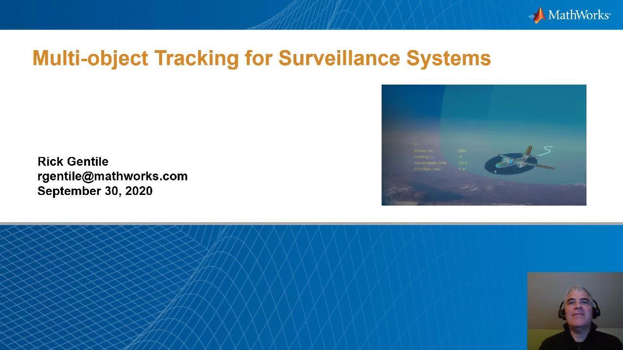
Multi-object Tracking for Surveillance Systems
Overview
In this webinar, you will learn how MATLAB and Simulink can be used to develop multi-object trackers for autonomous systems and surveillance systems. We will demonstrate how to generate complex scenarios to build a test bench that can be used to develop tracking algorithms. We will look at how to select the right tracker for your application. Through several examples, you will see how you can fuse detections or tracks from multiple sensors and multiple sensor modalities, including radar, lidar, and camera data. In addition, we will explore ways to measure the performance of the tracking system you build.
Highlights
You will also gain insights on:
- Tracking extended objects to determine size and orientation, in addition to kinematics
- Tuning trackers to gain the best system performance
- Perturbing ground truth and sensor configurations to increase testing robustness
- Testing tracking systems with Monte Carlo simulations
- Tracking objects in dense clutter
About the Presenter
Rick Gentile works at MathWorks where he is focused on tools that support radar, sonar, and wireless communications applications. Prior to joining MathWorks, Rick was a Radar Systems Engineer at MITRE and MIT Lincoln Laboratory, where he worked on the development of many large radar systems. His focus was on signal processing and system integration. Rick also was a DSP Applications Engineer at Analog Devices where he led embedded processor and system level architecture definitions for high performance signal processing systems. He received a B.S. in Electrical and Computer Engineering from the University of Massachusetts, Amherst and an M.S. in Electrical and Computer Engineering from Northeastern University, where his focus areas of study included Microwave Engineering, Communications and Signal Processing.
Recorded: 30 Sep 2020
Hello. My name is Rick Gentile. I'm a product manager at MathWorks, where I focus on radar and tracking products. I'm happy to be able to present this webinar on multi-object tracking for surveillance systems.
I'll focus on Sensor Fusion and Tracking Toolbox. This product was launched in the 18B release, and we just recently had a major update in the 20B release.
The toolbox has three major categories of capabilities. At the heart of the toolbox are algorithms for tracking, localization, and sensor fusion. And these are for surveillance systems and autonomous systems. We also provide a testbed that includes sensor models and scenario generation tools that you can use to develop and test your algorithms.
The third major category of capabilities is focused on analysis. And specifically, these are tools that you can use to visualize your results and produce metrics that you can use to see if your systems are performing as intended.
The Workflow is in place to help you work with data from your sensors. And this could be in the form of recorded data or data you feed directly from the sensor or sensors. You can generate this data directly from our sensor models as well.
We have a range of trackers to pick from that you can feed these detections. The interface to our trackers is through an object detections API. And our trackers produce tracks in the object track format. I'll talk some more about this in a minute.
Now, we took a two-design-point approach for this toolbox. You can use trackers out of the box or you can customize our trackers with libraries of tracking filters, motion models, assignment algorithms, and track fusers. You can also customize the trackers with your own tracking filters and motion models.
I should also note that the toolbox is written in MATLAB, so you have access to the code if you want to understand how we've implemented algorithms or how you might want to use it as a starting point for your own custom system.
So object detections can take many forms, as I mentioned earlier. We don't make any assumptions on what a detection is. You can define what a measurement consists of. I've included some common types here.
The top row shows what you might receive from a radar or a lidar. The point object would typically be seen for targets far away from a surveillance radar. For higher resolution radars, you may see extended objects where you get multiple detections per object per scan. Sometimes these types of extended objects can be clustered into a single detection. In the case of high resolution lidar, we can fit a 3D bounding box around the object and track the bounding box.
Now other types of measurements might include angle-only detections or range-only detections, and these types of observations typically require data from more than one sensor or data from a maneuvering sensor. We have an example that's referenced here that shows how you can map your own detections to the object detection format.
There are five sub examples that show various mappings that depend on the coordinate systems being used along with a sensor orientation, and this is all with respect to the platform's motion. I encourage you to take a look at this, especially if you have your own data that you want to map in to the object detection format.
When you have your own data, you can do what I just described. Even when you have your own data, though, it may be useful to use some of our sensor models to create test cases that form the corner cases that will stress your tracking systems. And so the sensor models we have fall into two categories.
It's important for any system that's doing multi-object tracking to know where it is in terms of position and orientation. So we have models that focus on the sensor positioning, things like altimeters and GPS and IMU, and also a higher level abstraction version for the inertial navigation system sensor.
We also provide a set of sensor models that you can use to generate detections to test your algorithms. This includes things like EO/IR, radar, lidar, and sonar. Object detections are generated from the sensors in the format that I showed you earlier.
Just a couple of examples here. For the radar, we have a monostatic radar sensor, and there are also some derivatives of this, some building blocks, that you can use to model multistatic radars as well as RF emitters, things like radar warning receiver scenarios. And the typical configuration is between 20 and 30 parameters that you can configure.
They all have defaults, so it's really easy to get up and running quickly. But if you have a radar that you want to model, you can go in and model things like where the radar is mounted, what it's scan pattern is, what type of scanning. It's also statistical in nature, so things like probability of detection and probability of false alarm can be used to quickly define a sensor. And the idea here is that you can take these sensor models and mount them on platforms, and platforms can be put together in a scene that allows you to create your test data to test your algorithms.
Everything that I show you here can also be done in MATLAB programmatically. But we also have an app that we call Tracking Scenario Designer that allows you to define platforms and targets. Then, you can also define trajectories. And you'll see, when I show you this--
Next, it's very easy to interact in the app and define your trajectories interactively. You can define sensors and add those sensors to the platforms, and then you have the option to generate sensor data. The good thing is when you're done with this, you can export this to MATLAB and get the MATLAB code to recreate everything you just did in the app.
We'd like to point out where you can use this app-- and also scenario generation in general-- to focus on these corner cases that will really show whether or not your trackers are working in the cases that they really need to perform. One of the typical cases we look at here is two objects coming together. In this case, two aircraft coming together.
For some amount of time, they fly parallel and then they go back out where they came from. And the idea here is that we're trying to create this region of ambiguity that often happens at long ranges in radars, where you have two objects, the radar sees it as one object for some amount of time.
In the Tracking Scenario Designer app, you can see that's exactly what we're doing here. This blue diamond represents the radar and it's going to be looking out in this field of view where we have these two aircraft. Right now, I've got one of the aircraft highlighted, and to generate this trajectory-- or just able to add waypoints in here that give it a trajectory. I do the same thing for the second plane and that's what you see over here in the yellow.
Note also the trajectory table and the time altitude plot. You're able to generate and change the altitude of the flight, either in a table version here or directly by just dragging these waypoints. This is a good example here, where I have it right-- This is the same piece, just pulling the waypoints down either in altitude or in the xy direction immediately changes the pattern. We can add another waypoint in directly in here and change the trajectory interactively. It saves a lot of time in terms of doing it programmatically.
I mentioned that there was a tower here-- and you see here that the tower is represented by this square object here-- and we can mount-- This is the bird's eye view looking down and this is the altitude version. You see that the radar here that we've mounted is on top of the tower.
The tower also has a sensor, and this is the sensor properties to find the radar that's been mounted on there. In this case, we've defined a mechanical scan, it's field of view. There's additional information in the detection settings for things like probability of detection and probability of false alarm.
When you're done putting together your scenario, you can run it, and you have two options to run it. You can generate detections or you can generate the motion of the objects that are going through here. You can see, as I'm pulling through, you're able to step forward and backwards and pause and really focus in on the corner case that you're looking to recreate.
And if you look over on the right side here-- Take a look at where those circles are. Those circles represent detections. And you can see where the two go into one.
We perfectly created the case that we were trying to, which is sometimes we have the two detections and then as they come together in that portion of the radar, sometimes we're getting the one detection. That's a case where we can see how the tracker actually performs in that scenario. There are many other kinds of scenarios that you can do the same thing with.
After you've generated the code in the app by hitting that export button, you end up with some code in MATLAB that when you run that code gives you the exact scene you just built in the app. One of the other things that happens is that when you look at the code that gets generated, you also see these comments that come out where you say "configuring your tracker here." You add a track plotter here, main simulation loop, update your tracker, and update your plotter.
And what I've done is I've just copied in the code that I added in to the code that was automatically generated from the app to show you how easy it is to add a tracker. We do some basic configuration. We initialize, in this case, our JPDA tracker. We set up the plotter. We set up the detection buffer, and then the small loop to process the detections through the tracker.
When we run this, we can see the same scenario we've just talked about. The beam is scanning, and you can see that there's two tracks there, track one and track two. You can see the full set of detections that have been generated. And now I've got this wrapped up in MATLAB code that I can use and extend in my test system.
I just introduced a tracker. We have multiple trackers that operate on those point object trackers. Remember I showed four types of detections on that top figure that I show here now, and I've grayed out the extended objects. I want to talk about that next. But if you look at the point object, the cluster detection, and the 3D bounding box, these are all potential inputs into these trackers that I'm showing here.
On the simpler end, the global nearest neighbor is there. And as we move down the table, we see things like the MHT and PHD trackers that are more computationally intensive, but they have strong roles to play in the tracking solution. So I'll show you and give you a sense of some of these in action. In fact, in the examples that are coming up, I'll show you a JPDA example and a PHD example.
We also have extended object tracking. This is, again-- just as a reminder-- when we've got more than one detection per object per scan. We want to be able to take those detections, put them into the tracker-- in this case a PHD tracker-- as well. And we're able to, in addition to getting the position and the velocity of the object that we're tracking, we're also able to get some sense of orientation and size. And that's important to potentially classify what you're looking at, or also figuring out where it is if you're trying to avoid it.
In the next example, I want to start with one of our point object trackers. To set the stage here, we've got four radars that are based on the ground looking up into space. Those white dots around the Earth you see represent space debris that we've generated orbits for.
And what you'll see is, as the debris passes through the radar coverage and detections are generated, those detections will be converted into tracks through the tracker. And as those tracks exit the radar coverage, the uncertainty of those measurements will start to grow until we get another measurement. And so, hopefully, that detection will be generated when it passes through the next radar.
Let's take a look at this. I just pre-recorded this just so you can get a sense of what's happening. It's easier to kind of walk through. You can see, just into that short portion here, the measurement was made inside the blue coverage and as it exited here and it's on its way through to another radar, the uncertainty of the measurement starts growing.
In the meantime, the tracker is predicting its next position here. You can see this continues. The uncertainty continues to grow. This gives you a sense of the global picture here, and you see the tracks coming out of the coverage each time here. You see T3, T8, T10. Those are ones that have already migrated through the field of view of the radars that we had.
What's nice about this is you can generate a scenario that would be hard to otherwise recreate yourself, and this allows you, in this example, to set up the radars, set up the trajectories of the objects that are in the field of view, and also test the tracker to see how they're doing.
In this example, we started off-- We could have actually used one of our off-the-shelf motion models. We have constant velocity, constant acceleration, a couple of different acceleration models, and also constant term. You could try to use these and play with the process noise, but basically, none of these match perfectly what an orbital motion is.
I wanted to include this here because this comes up-- this question comes up a lot about adding your own custom model. And in this example, we add a Kepler orbital model to describe the motion, and this helps the tracker predict where the object's going. So we get a detection and we're saying, well, these kinds of detections are going to be moving in this kind of a motion, and what's nice about this is you can test out your motion model directly.
And in this case, without adding a model like this, we would never be able to keep track of where the objects are. So I just wanted to show you that it's pretty straightforward to do.
This same kind of model, by the way, can be extended, and this small example here I'm showing we've kind of flip the problem where now the sensor is actually orbiting and it's looking down onto the Earth where the target is actually moving here. You can see as I rotate the globe here, the white sensor, that's the one that's looking down. You see the radar beam looking down at the Earth and the track being established.
So the basic simple piece here is orbiting sensor and track that's being generated directly here. And that's just a very simple extension to the first example I showed you.
In this scenario, we're going to have an aircraft taking off from an airport, and it's going to land at an airport in the distance. And we've got three air traffic control radars that are kind of monitoring this space. Sometimes we've got detections from one of the sensors, sometimes two, sometimes maybe three.
The idea here is that they're centrally tracked, so the detections are fed directly to a centralized fuser. We'll look at the performance of this system, and then we can compare it to the case where we take the radar sensor measurements in addition to ADS-B reports to help improve the quality of the track that we generate.
I'm going to start this video and you can get a sense of what's happening here. So the aircraft first takes off, and what you can notice is that we've got the path here where the detections are being generated, and you also see the track that was generated as a result of this radar data.
Once it achieves altitude, you can start to see the ground truth and the tracker start to match up a little bit closer. Those diamonds that you see there are the radar center locations. As this aircraft transverses and we sort of get up again to the desired altitude, and we finally make our way to the final destination and we're landing.
We can take a look at this whole scene as it's playing out and see how the system performed. We've set this up because we know ground truth, and all of our metrics that we show will be compared to the ground truth metrics that generate.
When we started the scenario, we just had radar and we're able to get radar detections every 12 seconds. That's the update rate of the sensors. And then, the second piece is we can rerun the system, but this time, in addition to the radar detections, we're able to add ADS-B detections. Those come in every second. So when we look at the metrics here, ground truth versus altitude, ground speed and heading, you can see how the system performs.
In this plot, the blue dash lines are the ground truth and you can see a couple of trouble areas here. The first one is that when we add ADS-B into the sensor, you see a much improved performance on the altitude estimation, where that green arrow is pointing. You can see this line is actually the surveillance radar only, and then the case when we added ADS-B, we bring it right up to the ground truth.
There's also a similar improvement for ground speed and heading when we add in the ADS-B, and this is primarily due to the update rate of ADS-B. The 12 seconds versus every second we're getting at this point.
These are the kinds of things that you can use not only to build your tracking systems, and you can really architect at a system level because you can tell how often the data updates have to come in. That can help drive your communications pipelines between these kinds of systems. So there are a lot of important aspects beyond the tracker, although the tracker is a key element of this and figuring out how to tune it and how to figure out how to best build up your tracking system.
In the next example I want to show you, it sort of builds on this. We're going to use a tracker but we're also going to extend how we do the data generation portion. We'll start off again with a lat-long altitude based trajectory. We'll use that trajectory as the baseline to form multiple trajectories. We'll do that by perturbing the parameters of the trajectory within some confines of some bounds that we want to put in our test system.
And then when we're done with that, we'll use that information to generate scenarios which will generate detections that can be fed into trackers that we develop. We can see how the tracker does and if it's able to correctly identify tracks that were anomalous and tracks that were nominal.
Now in this case, we'll define the detection of an anomaly as one of these trajectories that go outside these black squares or rectangles as you see approaching landing. So the aircraft's coming in. That cyan line is a trajectory that we're going to use as our baseline, and those black rings around the trajectory identify when an anomaly is present.
So we do this. This is pretty straightforward to do. Just give us some waypoints. We generate the trajectory, and we're going to use that with our sensor model that models the airport radar.
We can define the perturbation parameters. You see that on the bottom. The waypoints are perturbed with a zero mean normal distribution with a decreasing standard deviation. These are just for this example, but you can make up your own perturbation parameters.
When we generate-- We started with that one trajectory and we're able to generate multiple trajectories, and this is the code that's required. The perturbation starts with the baseline approach trajectory that's defined by the waypoints, and we're perturbing those waypoints around the parameters that I show you on the bottom of the slide here. We put this in a loop and then we're able to generate more than one set of data. In this case, we have 20 trajectories that we're using. This could be whatever number that you want to use in your test. In the picture, again, yellow is anomalous and cyan is the safe trajectory.
And so, when we're done, we're able to feed in those trajectories into a scenario. As part of the scenario, we have the platforms that are moving. These are the aircraft. Those are targets essentially to the airport radar.
You notice the pink dots that are popping up? Those are false alarms. So we can model that in the monostatic radar sensor model. And we're able to kind of complete the loop by saying, well, OK, I've generated data. I used that data to feed a tracker. Then I can measure the tracker performance against how it did against ground truth. In this case, there were actually seven anomalous trajectories out of 20, and the tracker was able to get the correct answer in this scene.
I want to leave you with that point of being able to, again, create a test case-- in this case, with perturbation technique, you're able to generate one and transfer that to many around some perturb set of either trajectories or even sensor models. For example, that same technique can be used in the sensor model where you're trying to vary the types of parameters that might change across different sensors.
My last example here on point object trackers is using the Gaussian mixture probability hypothesis density tracker, GM-PHD. The scene here is that we have a high clutter seen, very dense clutter, and there are actually some targets in here. If you look at it closely, you probably can see them. There's actually five objects in here.
The thing about this is that from a sensor model standpoint, back to the monostatic radar sensor, by just increasing the false alarm rate, you can generate this type of clutter for your test purposes.
I mentioned phased array system toolbox earlier. We also have clutter models if you're modeling at the IQ level as well that you could use. But in this case, I'm using the statistical model.
I turned false alarm rate-- false alarms on and I've given it a false alarm rate that I can vary to increase or decrease the amount of clutter. Here's with a tracker on. You can see, there were five targets and the tracker picks them up, one through five, and you get a sense of how we do this.
The one thing I want to point out on this tracker is that this kind of a scenario would be very tough for one of the other traditional trackers, the GNN or even the MHT or JPDA. It would bring it to its knees, this kind of a scene, because it would try to establish tracks on all of these guys and it would really slow down.
Again, that just depends on how dense the clutter is, but there are some parameters in this tracker that allow you to say how many detections you expect to see per object. That's something you'd have as your system knowledge. In this case, we're saying one, so this makes this tracker operate as a point object tracker when it's configured to one.
And we also have this concept of the birth rate, which allows you to control how a track is established here. That's one of the big differences between this tracker and some of the other traditional trackers that we have, that you can pick this and this is why it performs well under these kinds of circumstances.
I've got a couple of examples here that I've included to highlight some of the metrics we have. And one of the newer metrics that we've introduced is called GOSPA. What's nice about the GOSPA is that it's an integrated metric. It has the traditional kind of components, things like missed targets and false tracks that you would think of when you think of multi-object tracking. But the beauty of GOSPA is that it also gives you this integrated metric score that has an integration of all the building blocks of the metric.
This is nice for Monte Carlo analysis because you can just look at the single value and see if it's good or bad. In this particular case, the top plot, lower is actually better. And you'll see this in a couple of the examples that I show coming up.
Speaking of Monte Carlo, we can run this again, this kind of same scene, and look at the GOSPA metric across these different parameters. In this case, we're using probability of false alarm as a varying parameter. And, as I mentioned, in the monostatic radar sensor model, the PFA is what actually generates the amount of clutter.
You can see how this tracker performs at different levels of density, of clutter. It's quite useful in that sense. Hopefully, you start seeing the theme here of being able to test your systems and be able to make them more robust.
I just showed a PHD tracker being used as a point object tracker in that dense clutter scene, but the same type of tracker can be used for our extended object case. Showing you that ship again. I'm going to go into that in more detail next. But the idea of this tracker class is that you can use arbitrary shapes-- this could be rectangle or elliptical-- that allows you to try to estimate size and orientation in addition to position and velocity.
We have clustering algorithms that you can use, and there's a variety of these kinds of clustering algorithms. We have something based on DBSCAN that allows you to cluster your detections.
In this case, we've got three ships and we're actually clustering in the different colors there. The red, yellow, and purple are actually being generated with our DBSCAN. This can work, and you can use this technique to feed the PHD tracker. You could also use this to once you have the clusters actually translate this to a point, maybe it's the center of gravity of the object, and those could be put into point after trackers.
But for this example, I want to take the cluster of detections and feed them into the extended object tracker. Let's look and see what that looks like.
In this example, the radar is in the top left, looking down towards the bottom right, and we have the three ships. You can see there are two small ships and one large ship. And in this particular example, we're actually using the ellipsoid as the shape estimate.
So what you'll see is-- a couple of things to note. When object three, that one at the bottom, goes in the shadow of the ship, you can see that the detections are lost. Watch as it repeats here. It gets to the back and it'll start to come here. These red dots are detections. As soon as it goes behind the shadow of that ship, the detections disappear. And as soon as it comes back out, you'll see the detections again. That's what results in that little imperfection in the route or the track prediction of where it was in the shadow there.
The other thing I want to note is that those ellipsoids are actually predictions of the shape of the object. We also have versions of this, as I said, that you can use for rectangular shapes as well and you get a little bit more accurate answer.
In this example in particular, we're modeling a 2D radar, so if you look at the ground truth of the large ship and the small ship versus the estimate, some of them are pretty close. They're in the same ballpark. You certainly can see small ship versus large ship.
Because it's only a 2D radar, the height is a little bit off. That's understandable in this case. And then, also, because we're using the ellipsoid in this example, the measurements aren't perfect. But the idea here is that you have some sense of the extent of the object. And that can be useful, again, for classification. It can be useful if you're building an autonomous system that you want to figure out exactly what direction it's heading in and what its orientation is so maybe you avoid it or you again help classify what you're looking at.
We can track extended objects with lidar, and one of the options that we look at sometimes is taking that lidar, that high resolution lidar, fitting it with a bounding box and then using that bounding box not as an extended object but as a single object that can be fed into a tracker like a JPDA, MHT, or GNN. That's certainly a valid technique, and we have a lot of examples to show how to do that. But we can also actually treat it as an extended object and feed that into the extended object tracker. This is what this next example will show.
Kind of sticking to the airplane theme a little bit, imagine the aircraft is now landing at the airport and as it pulls into the tarmac, a couple of things are happening. The service vehicles are going out and the personnel is coming in to service the aircraft. That's kind of the starting point.
I mentioned the monostatic radar sensor. We have a corresponding one for lidar. And this, again, is just there for test purposes to generate data that you can use to test your trackers. Now I've got the tracker kind of enabled here. So in this case, it's again the PHD tracker and you can see the numbers now. Those represent tracks. And on the right, I'm showing you the GOSPA metrics. The missed target again, false tracks, localization, and the integrated score. Again, integrated score one is lower is better.
What you see is-- The first thing you want to look at is, well this time, we didn't have any false tracks, just like the other example I showed you. But in this case, we actually have a missed target and it happens twice, at the beginning and at the end. Let's take a look at those.
The green arrow here is pointing to track 11, which takes a little bit of time to actually get created. Of course, we have the ground truth, we're comparing to the ground truth. So we know in that initial section there, the object is actually too far away from the lidar and it's not being detected until it comes a little closer. Then the track has formed, and then this value goes back to zero here.
We go for some time, and then our system says that we're missing another target. That is actually from our track five and we start off-- Here, it's the opposite. We start off with a track, because it's in the lidar field of view. But as soon as it goes behind the shadow of that aircraft, we stop detecting it and then we have a missed target.
Again, I keep going back to the theme of creating the scene, getting these corner cases, and then being able to evaluate with metrics to see how it's working. The systems I've shown so far, for example that aircraft one that's transversing from takeoff to landing, I had three radar sensors and I had-- second I added ADS-B, and I was able to fuse those detections at the central level. I put out tracks that we could evaluate.
The key theme here is that this usually will give you a better answer. It'll give you more accuracy. This can be with one or more sensors. I showed a couple of examples here where we had one sensor doing it and the case, for example, air surveillance radar with the three radars and ADS-B sensors feeding in. This can be more than one target, and this can be a combination of point or extended objects in the system.
This little graphic here I show-- I did this in a past webinar, but it's basically three sensors, two aircraft, one on the ground, and then seven objects in the field of view. That's an example of where we're sending the detections to a central location and we're fusing them to get a better answer.
The alternate approach is to actually send tracks from each of the individual sensors and fuse them at the central level. This example is really about taking sensors in, putting tracks out, distributing those tracks to a central track fuser, and then that's where the track assignment is done in the central-- track update is being done on that track fuser.
In this case, we think of-- this could be an autonomous system with a lidar and a radar on it. It could be UAV with the same kind of sensors. This could also be a system of systems where you have multiple radars and EO/IR systems feeding track information to a centralized tracker.
I want to show you an example here. I'll use this radar-lidar fusion example to explain the concepts. But the idea here is on the left. You see I'll have two track outputs from different sensors and when I fuse them, I still get, hopefully, a better answer than what I had if I just had a single track. That's not always the case depending on the correlation of the sensors, but that's the goal.
I think the key benefits here are really focused on maybe lowering the bandwidth between the different sensors in the central fuser. Also, the diversity of sensors can also drive the need for optimized trackers at each of those sensors. So in some ways, that's a benefit because you can-- the tracker that you use for lidar may be completely different than the one you use for radar, so you're able to sort of mix and match and optimize the tracker selection at each of the end nodes.
Of course, the more processing you do at the end nodes, the less you potentially have to do with the central node. In a lot of these cases, it's just a way to standardize the interface across disparate sensors, right? You can do this and say, just give me a track list and I'll process it. It helps standardize potentially in an autonomous system or a system of systems as well.
The downsides-- I mentioned accuracy already. If you have detections, you're getting more information, and you put those together and you'll probably get a higher accuracy.
There's also the concept of correlation noise where if you've got multiple sensors that use all the same types of techniques, getting two different measurements or two different tracks from those kinds of sensors may not actually improve the performance of anything.
The other concept, the last concept, is rumors. We have an example that we do to show how to manage rumors, but think of rumors as a case where one sensor sees the object and at some point it loses track on it, but it's sharing its tracks with another sensor. That sensor starts tracking it, and at some point neither of them see it. The risk of a rumor is that while neither of them see it, and it's not actually there, they're still reporting it. And so we have some capabilities in the trackers to help you avoid that in your system.
Let's get back to this example here. We start off with the autonomous vehicle. In this case, the ego vehicle has lidar and radar, and this is just the picture of the ground truth. The green dots are the point clouds from lidar and the blue circles are detections from the radar. This is a little bit sterile. You can see some false alarms here, but we're just trying to keep it simple to start with because the concepts are very similar.
Leveraging what I talked about earlier, in this case, we're using the 3D lidar to generate bounding boxes. Those bounding boxes go into a point object tracker, in this case JPDA. The 2D radar is actually taking those unclustered detections, those blue detections, and feeding them into the PHD tracker processing extended objects to tracks. And then we're fusing those tracks to get a better answer than we would get otherwise.
What happens is-- The bottom right one is the one to pay attention to here. The F is the fused track and the L is lidar and R is radar. What you can see is, most of the time, the lidar will actually be better performing because it's higher resolution. But in that case that just happened-- and watch it again, I'll show you a little bit clearer-- when the two cars go by, the lidar tracker actually keeps-- I'm going to just play this again-- While the two vehicles pass each other, you'll see the lidar track sort of migrate to right there.
That's a problem. If we didn't have radar there-- The radar has much better information because the radar detection includes a range rate information that the lidar track doesn't. And so, what you'll see is that the answer that you get by the fuse system is closer to ground truth than if you just look at any individual sensor.
Again, the closer look here is the ground truth is two vehicles together. The radar is not perfect, but it's much closer than you'll see the lidar is. The lidar migrates through here, there's confusion, and if the system was just using lidar, there might be some trouble, especially in an autonomous system where the margin for error is much smaller. When you put the fused one back together again, you're getting the benefits of what the lidar shows plus the radar shows and you get a better answer.
I want it come back to GOSPA again. The GOSPA is a combination, again, of the position error, the missed truth penalty, and the false track penalty. And here, again, lower is better. This is the integrated one for the example I just showed you.
Remember, I said, in general the lidar-- once the track gets initialized, the lidar should give you a better answer. So here, lidar is this red color. And you can see, in general as it's coming through here, in a lot of cases it's much better than the radar, which is in blue.
The other thing to point out is this note here, is that as you'd expect, the fused answer is better than any individual sensor. That's good. That's why we're doing sensor fusion.
That case where I showed you where there was trouble, where the lidar segmentation was incorrect, it produced a large position error. And that made the score for lidar increase. In fact, it increased above the radar where we actually use the radar information more than this system.
Before I end up here, I just wanted to highlight that all the detections that I showed you up until now have been those point object ones or the extended ones from radar or lidar, where we're getting a complete measurement. But also, it's very common in surveillance systems to have angle-only or range-only measurements.
Again, the common theme here is that typically you'd have more than one sensor that you're fusing, or if you only have a single sensor that has a passive mode, you need to be able to outmaneuver the source of the emission.
This example is one that we have that I just want to call your attention to in case you're interested in this. There's a lot of information on our website about this. But basically, it's multiple synchronous passive sensors where we feed in those detections, those angle-only detections, into a static detection fuser. Take the output of that and feed that to one of the trackers I talked about earlier in the session today.
In addition-- Just like the other examples I mentioned, in addition to being able to figure out how to configure the tracker, you also can figure out system bandwidth issues, sensor location concepts. You know, where do we put the sensors? How many sensors do I need? How good do the sensors have to be? Those can all be done. What kind of communication path needs to exist between these sensors?
Similar discussion for range-only. I showed you that monostatic radar model, and the building blocks that you can also put together to form a multi-static system. Those are also in place. Here, you can see on the top we're finding these domes that basically represent where a target could be. And when we look at those across the four receivers we have, we can actually focus down exactly where the target is. And this also works for multi-object scenes too.
The last one I want to mention is when you have range-only and the sensors are not synchronous, you need to bring in filters like the Gaussian sum filter or particle filters to help with this kind of scenario to figure out where your objects are. These are all options. These are all ones we have great examples to get started with if you're interested in this type of workflow.
This session wouldn't be complete without me reminding you that with tracking, we have the nice advantage that you can actually generate C code. And with a C code generation, it greatly speeds up the simulation time. It also gives you a head start to deploy your prototypes or even your end system.
I encourage you to take a look at MATLAB Coder, and with MATLAB Coder-- these examples here generate C code. This one that I'm showing you here on the right is 1,000 objects moving in a flock, and the one on the very right is just a zoomed in version of this flock. We generate C code and the speedup is pretty dramatic, 40x is not a possible speed up during this time.
Let's bring us close to the end here. I just want to remind you, most of what I showed you was Sensor Fusion and Tracking Toolbox. Of course, the ones that were related to autonomous systems and automated driving, we also use the Automated Driving Toolbox to set the scene up and build up the scenario that we used.
There are also a lot of other resources to get started with. We have a couple of e-books that you can download that go through everything from multi-object tracking to sensor fusion. Our product page has a lot of great information. We also have a "Getting Started Guide" to help you select tracking filters and trackers.
And we've also got a series of Tech Talks that really span the topics of sensor fusion, localization activities, the IMU GPS accelerometer, things like that. And then multi-object tracking including extended object tracking and track-level fusion. I encourage you to take a look at these. There's a lot of great information in them.
With that, I thank you very much.
Featured Product
Sensor Fusion and Tracking Toolbox


Seleccione un país/idioma
Seleccione un país/idioma para obtener contenido traducido, si está disponible, y ver eventos y ofertas de productos y servicios locales. Según su ubicación geográfica, recomendamos que seleccione: United States.
También puede seleccionar uno de estos países/idiomas:
América
- América Latina (Español)
- Canada (English)
- United States (English)
Europa
- Belgium (English)
- Denmark (English)
- Deutschland (Deutsch)
- España (Español)
- Finland (English)
- France (Français)
- Ireland (English)
- Italia (Italiano)
- Luxembourg (English)
- Netherlands (English)
- Norway (English)
- Österreich (Deutsch)
- Portugal (English)
- Sweden (English)
- Switzerland
- United Kingdom (English)