Predicting Boiler Trips with Machine Learning

Good day, and thank you for joining us on this webinar on predicting boiler trips with machine learning. This project was a collaboration between Opti-Num Solutions and John Thompson boilers. My name is John Atherfold, and I'm a data science specialist at Opti-Num Solutions, working specifically with our smart mining and manufacturing focus area.

And I'm Christopher Van den Berg. I'm the cyber physical systems engineer at John Thompson within the industrial watertube division. I mostly handle the research and development projects there. In terms of the contents of today's presentations, we'll be giving a bit of background about both companies and the project itself, and why it's important, and why you should care about it.

We'll then dive into the solution workflow that was implemented using MathWorks tools. And finally present some results of the deployed application and our summary and conclusions of the project. So just something you should know about John Thompson, they're a global provider of boilers environmental solutions, engineering, energy management, manufacturing, spares, maintenance and training. They're a part of a division of ACTOM. And ACTOM is the largest manufacturer, solution provider, repairer, maintainer and distributor of electromechanical equipment in Africa, also a major local supplier of electrical equipment services and balance of plant of renewable energy products.

Before we dive into the project background, I'd like to talk a little bit more about Opti-Num solutions. Opti-Num was. Founded in 1992 as the sole distributor of MathWorks tools in Southern Africa our business evolved strong-- a strong services approach ever since 2015.

We are currently a level 4 BBBEE contributor. And our clients include many of the JSE top 40, including but not limited to PowerProtect Transformers, Anglo American, and Sasol. Our smart mining and manufacturing team is focused on unlocking profitable insights and solutions to real world problems using your process data. These solutions could include advanced data visualization, smart monitoring and maintenance, as well as intelligent control.

So the first application of boiler trip adivsor was actually at a sugar refinery. And one of the byproducts that is heavily used to fill boilers is the gas. So the gas is basically the plant fiber that is left behind after the crushing.

And it's normally this high energy, dry biofuel that can be useful to power boilers. And it actually garners about 5,000 to 8,000 BTU per pound of the gas. So it's a lot of energy condensed into that.

So when-- from the boilers, they use the gas to fill the boilers. And then they produce steam. And then two types of steam that they produce is the processing steam, which is saturated steam.

And they use that for cooking and drying the sugar cane. And also use it also to make superheated steam, which is used to fuel turbines to produce electricity, or it is used to power some of the machinery in the process. So on the site, we redeployed the algorithm.

They had two industrial water tube boilers that were bagasse filled. And the first one being an any time per hour boiler. And the second one being a 50 temp per hour boiler.

This became our testing ground for boiler trip prediction. And this works out because there are two different types of boiler trips that can generally occur. The first one being excess might occur in the FDL and defense.

And when this occurs, it's likely caused by a blockage in the flue- flue gas flow. And when this trip occurs, it actually is done in order to protect the furnace pressure and also exceeding the excess heat in the furnace. So if the furnace pressure becomes positive or too much, it can cause damage to the firing arc of the boiler.

And if there's excessive heat in the boiler, it can cause too much heat being transferred to the stoker, which can cause damage to the stoker. The second type of boiler trip can occur on the water level switch in the steam drum. And either this occurs when the water level is too high or too low in steam drum.

So if the water level is too high in the steam drum, it can cause water to enter the superheated steam that goes through the turbine. And if this occurs, it can cause water to get onto the turbine and cause corrosion within the turbine. The second type-- when the water level is too low on the steam drum it causes the water in the tubes of the main bank and that causes it to dry out, which means that all the heat that is transferred from the amplifier to the tubes will go directly to the tubes instead of to the water. And this can cause warping and damaging to the tubes itself.

So a little bit of background on the project, and why it was necessary, and what the exact application of it is. So first off, let's address the challenge. Boilers are process critical equipment.

And boiler trips result in unplanned downtime for any production process. They can-- boiler troops can seriously cause significant loss of production in the mill and reduce overall throughput of a time, over the day or over the month. So what we did to address this challenge was we implemented an early trip detection system using tags that we found upstream of the boiler.

Our detection system warns the operators of impending trips with enough lead time such that the trips may be prevented. The final result of implementing this algorithm has been fewer trips on average per month and an increase-- an overall increase of plant production due to the decreasing frequency of boiler trips. You may be wondering what the final solution will look like and how it integrated with existing aspects of the plant.

So initially, we have data-- sensor data that is streaming in. And that is ultimately fed into our historian. From there, the historian data is accessed by our executable file, which is sitting on an existing server or an existing edge device that is on the plant.

The server then writes information back into the historian. And ultimately, we could analyze these results over time and see how many boiler trips were prevented, and also evaluate the accuracy of the algorithm that had been implemented. In terms of what this executable file consisted of and what it looked like, it was a Matlab application that was developed in App Designer and-- well, developed and deployed as an executable from App Designer.

And ultimately, there were several aspects to this executable file. We'll dive into each of these aspects individually in a moment. So first up was data access.

So the executable file had to access data from the historian. Then it happened-- then some data pre-processing happened, which consisted of mostly two steps of data pre-processing. The data-- the pre-processed data was then fed into-- the live data was then fed into a machine learning model.

And finally, the results were visualized in a graphical user interface, or GUI. The first aspect of our solution that we'd like to discuss is how we access the data. And this was done via OPC For those of you who are wondering what OPC is, OPC stands for open platform communications.

And it is an interoperability standard for the secure and reliable exchange of data in the industrial automation space and other industries. We are typically operating in this blue circle over here, which is taking data from physical sensors on the plant, moving them through the DCS, distributed control system, and ultimately pushing them to the historian. And we access the data from there.

But as you can see, there's a wide breadth of application for OPC in general that spans entire-- that could potentially span entire operations, including pushing data to the cloud or exchanging data with the cloud. Why did we use OPC? It is the industry standard and hence, it's tools agnostic.

So it doesn't matter what type of PLCs are being used or what type of historians are being used, we are still able to access that data. And it allows for access to live data and historical data through any historian. We also used Matlab's OPC toolbox quite extensively in accessing the data. And this was a very user-friendly route to take.

For this particular project, we were interacting with OSI PI-- an OSI PI historian. But as I said before, we could-- Matlab's OPC toolbox can interact with any historian. We integrated using the historical data access server, but we could also-- it's also available to integrate via just the data access server and the universal access server.

Now, discussing the OPC toolbox in a little bit more detail and the exact workflow that was followed. So the first thing we need to do is locate the OPC server on our host machine. And that allows us to examine-- yeah, examine the structure that's returned in slightly more detail that provides us server IDs.

And from there, we can decide on which server or servers we would like to connect to. From there, we create our OPC client object. And the object is created using the hostname and the server ID that we'd like to access.

From there, we connect to the server, which is done with one line of code. And this needs to be done before accessing any data from the server. After that we create an OPC group and that helps us manage the particular tags that we would like to-- that we would like to gain data from.

So these groups contain a collection of data access or historical data access item objects. And they're effectively used to control the items, read values from the servers and manage logging tasks. From there, we would browse the item namespace.

And that allows us through Matlab to search the available items on the OPC server. And we may-- and this is done because we may only want to access particular items on the server. We would then add the items to the group.

And this allows us to easily read data from multiple items by calling functions on the group instead of the individual items. And finally, what we would do is read the data directly into Matlab. And we can do this either in a raw form or in some sort of pre-processed form.

The next step in our solution workflow is data pre-processing. And as mentioned before, there were two main stages to this process. So as data-- as raw data is read in from the historical data access server, it's in a state that's slightly jumbled up and needs a little bit of cleaning before we proceed.

So the next step here is to sort, fill and re-time the data into a timetable object where it's easily interpreted and easily accessed. From there, we move onto our feature engineering where we take our features and general-- well, take our raw tags and generate some features from them that are able to be fed directly into our machine learning model. The first step of data pre-processing was sorting, fulling, and re-sampling our raw data.

And these very basic data pre-processing tasks are made easy by using Matlab's built in functions. So the first thing that was done was the data into chronological order because, as mentioned before, when it gets returned from the historical data access server it can be in a slightly jumbled up state. The next thing we did was find and remove repeated times.

And from there, we filled in any missing values. We typically used a cubic spline in tabulator for most cases. But in cases where this wasn't possible, we filled we filled the data in using the last or the previously finite value of that particular tag.

And finally, we re-sampled the data-- yeah, we sampled our processed data to a regular sample rate. The next step of data pre-processing was engineering our features that enabled us to feed our information into our machine learning model. The first thing we did was define what we called a reference table.

And this was a table containing plant data from where the plant was stable and operating normally. So how we did this in particular was we took a look at some period of time and through the historical data access server, and accessed I think it was the last few days worth of data and from there, defined periods where the plant was operating stable and normally. And this became our reference table.

Next we defined our query table. And this was a table containing the most recent plant data. And this was effectively compared against our normal-- our reference table using our machine learning algorithm.

In addition to this, we did several transformations to the data. The first of which was a different table, which gives an indication of instantaneous rate of change. And that was as easy as calling the diff function on our table.

The next, we detected the trips in data chunks if they exist-- if they existed or if a trip occurred using an indicator tag that was indicative of a trip happening. And finally, we centered and scaled our data appropriately before further pre-processing The next step in our future engineering journey was running our data through a principal component analysis or PCA, on both training and testing.

And this was physically done was we ran the principal component analysis on the training set initially or on our reference set. And then onto those principal components, we projected the data from our query set. We've done in this way in order to prevent data leakage.

And ultimately, if we took our first three principal components and visualized them for our analysis data, we had this plot. And what we can see with color is our first, second, and third principal components on a 3D scatterplot. And if we colored them accordingly to how close they were to the trip, we could see some interesting features coming out of our principal components.

The one noteworthy thing is that most of the normal data is centralized in this centimeter cluster. And as we get closer and closer to a trip, there is substantial deviation from this cluster. And ultimately, we thought we could start-- well, we thought we could use this distance as a feature, as a potential means of predicting when a trip would occur.

So that led us to getting the Mahalanobis distances of the training tests-- training set and the testing projection. And that effectively quantifies the deviation from normal, or it is one potential way to quantify the deviation from normal. And if we take a look what those distances look like and we plot them on a histogram, we would-- it would look a little bit like this, where the blue histogram with its median is sitting over here, and the orange is-- and that represents our training data set or reference table.

And our testing data set or query table comes in like this and is, as we can see, a little bit further away from our-- from our reference data set. These types of plots and these histograms and properties of these histograms were used in engineering further features that fit into our machine learning algorithm. So in a similar manner, we generated other various statistical parameters, and which include the median, the interquarter range, rates of changes of various parameters, the KL divergence, and the skewnesses.

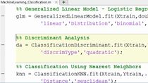
These features ultimately describe various properties of the normal operation data set, the incoming query data sets and the differences between them. And it is exactly these types of differences and this information that we would like to map back to when trips would occur. Next up on the workflow, we have the machine learning model itself and details around how we formulated the problem to fit into a machine learning workflow.

So our initial plan was to pull the regression model able to predict the time until trip, or TUT, similar to how remaining useful life models work and remaining useful life predictions in predictive maintenance. The end product was a classification model that classified chunks of input data into one of five classes. The first class was that the time of-- time until trip was greater than 40 minutes away.

And this ultimately indicated that the chunk of data is healthy. The next four classes are a success of states of degradation and as our boiler approaches a trip. And our final class is that the time until trip is less than 10 minutes away. And this indicates that the chunk of data is very unhealthy.

And that the trip is imminent. Each of these classes has a probability associated with it. And the probability distribution associated with each chunk is rolled up into a single health value for that chunk of data.

The final machine learning model that we used was a boosted forest. And this consists of a series of decision trees. And effectively, what we're doing is we're creating an ensemble of-- an ensemble of weak learners.

And this is typically known as ensemble learning. A weak learner is a type of machine learning algorithm that typically doesn't perform very well on its own. And it either typically over fits or under fits, depending on the context.

The idea behind having such an ill-m suited learner in ensemble learning is that if each of the different learners are trained on a slightly different set of data or trained in a slightly different way, then they're able to individually make bad predictions but together on the whole, on average make really, really good predictions. So a brief illustration of what a boosted forest looks like. If we consider a single decision tree in which the full data set is fed in and a series of decisions is made, and ultimately a final decision is made, which constitutes which class that our data set ultimately belongs to.

How a boosted forest works in a slightly different way is that we feed our full data set into our first tree. But instead of a classification getting output, we have an adjusted data set. That adjusted data set then gets fed into a secondary, out of which appears another adjusted data set. And this tree is trained slightly differently from the previous tree.

This continues until finally after a number of trees, we have a decision. And this is, yeah, this is what a boosted forest looks like. This is slightly different from a bagged forest, which I won't go into during this presentation.

How we fit an ensemble tree in Matlab is simply by calling this fitcensemble, that's fit classification ensemble function, on our data. And into this function as arguments, we're going to pass in our training data table as well as the name of the variable in the table that is our response variable. The hyperparameters, there are many hyperparameters associated with this model.

And all of these were tuned by a process of Leave One Out cross-validation. And how we did this was by using the cvpartition function in Matlab, where we specify how big our table is and then effectively just specify the leave out function. And what's returned is an object that partitions our data in whichever way that we request.

Subsequent hyperparameter sets were chosen using the Bayesian optimization function. And that exists in the statistics and machine learning toolbox. And effectively calling, that function looks a little bit like this, where you called bayespot, and you get a result structure in return.

Arguments to this function include a loss function, which needs to be specified, as well as the entire set of hyperparameters that need to be passed into the model. The hyperparameters are passed into the fitting function as name value pair arguments. The first thing we need to specify when specifying an ensemble or one of the things we need to that needs to be specified is the type of tree that is used.

And we can specify this by calling the temper-- calling the templatetree function and specifying our hyperparameters, such as maximum number of splits, minleafsize, and what-- and the split criterion that we're using. This entire tree along with other types of parameters will get passed into a classification ensemble learner, as well as the method learning rate, number of learning cycles, and so on. Predictions are made on oncoming-- on incoming query data using the predict method.

And that's as simple as calling the predict method on our trained model. The group that's returned out of our predict method is the actual classification. And scores is the probability associated with each of the five classes that are used to calculate our health value.

This model was trained and validated on just over two years worth of boiler trip data. The final part of our solution is the development of our GUI, or graphical user interface. This, too, was built in Matlab using an object oriented programming approach as well as App Designer.

This was deployed to an etch device as an executable using Matlab compiler. The architecture we followed to develop the GUI followed a variation of the model view controller framework or MVC framework. And that looks a little bit like this, where the user would the user would use the controller, and the controller in turn manipulates the model, which then updates the view.

And then the view displays whatever the update is to the user. A controller class coordinated all other aspects of the framework, including the Data Manager class, which was responsible for the communication via OPC. And it was responsible for saving out-- saving our data and saving our error files.

The model class contains the machine learning model and some of the future engineering that was required to pass-- to create the features from the raw data. The view class displays information to the user. The intention of this was to provide information to operators, informing of them-- informing them of potential trips so they could take action and prevent downtime.

Refinements of this workflow involve integrating directly with existing HMD on the plant as opposed to having operators viewing a separate application. We'll now take you through exactly what the GUI looked like and the type of information it was able to display to various different viewers. This is a snapshot of the GUI as it's operating live on site.

As you can see, it consists of three tabs-- the server tab, an advisor tab, and a details tab. On our first tab, the server tab, we could take a look at the status of the boiler trip advisor. And this was to indicate errors or successful-- or successful or unsuccessful connections to the various OPC servers.

In this block over here, we can see that OPC server details, which connects both to the data access server and a historical data accessible. And finally here we see information of data packets from the last 10 minutes. And you can see that it's approximately in the same form as a data timetable, which is indexed by time.

And each of the columns represented a different tab. The second tab on our GUI is our advisor tab. And this contains high level information about the state of the boiler. So the first one is-- the first block is a prediction of the trip.

And a long-- well here, we can see there's a probability of a trip as well as an indicator time until trip. The second block over there are the tags with the greatest health value impact. So effectively, what's done is a feature importance analysis.

And from that-- out of that analysis comes a list of tags. The intention behind this is potentially extending the advisor with a root cause analysis such that the advisor would be able to tell the operators not only when the boiler would trip, but which tag exactly is causing the trip. Finally, we have a trendable health value that gets plotted over time.

And this allows the operators to view the current health state-- health state of the boiler as well as which direction it looks like the boiler is going to be headed. The final tab of our GUI is the details tab. In the details tab, we can see a little bit more lower level information on our political advisor and the predictions it's making.

So over here on this panel, we have detailed trip and data packet timings. So-- well, it's detailed trip information and data packet timings. So effectively, we have the probabilities associated with each of our five classes as well as the timing details, so it tells us when our next test of time is expected.

So we know when to expect an update to our plots and an update to our health value. Finally, we have a boiler status panel, which indicates the current class-- yeah, the current classification that the algorithm is made, as well as the exact health value. And as always, our health value trends remain. So we'll now go to Christopher to see some of the results of the boiler trip advisor in action.

So where we had the BTA deployed, we had it on trial for about three weeks while normal operations took place. From the data, the following events were of note. There were two cases of a successful production of a boiler trip.

So this is where the BTA specified that there would be a trip before a certain amount of time will occur before the actual trip occurred. There were four cases of a successful prediction of a let-down event. So let-down event is where steam is passed from the superheater to saturated steam to other parts of the processing.

And there were three events of an undetected event or trip, just false negatives. There were also 14 cases of false prediction of events. But this may have also been events that were intervened by operators.

So on this slide, it shows table of the data from week 1 of the trial. And it shows that a lot of these events occurred when the health value was below 0.5. It also shows the time where the BTAs triggered these events.

And it also shows where the actual time of these events occurred. And if you look at the time discretion between the BTA and the actual events, you can actually determine how early the BTA predicted the events. And in this one, it shows that there were three successful predictions of let-down events.

There is a graph just indicating-- showing off how the BTA reacts in terms of a let-down event. And you can see that as the health value declines, it can already see that there's going to be a let-down event occurring. So on the graph, the blue line represents the health value.

And on the orange line represents the let-down valve position. So as the health value decreases, there's an indication that there's a deterioration in the boiler's health and that let-down-- the let-down valve will need to be open for a let-down event. So here is a table of the results from week 2.

This table shows pretty much the same data offered back-- shown in the previous slides. On this week, we managed to have a successful let-down event and a successful trip event. So on the next slide, I show you-- I'm showing a graph of how the interaction of the BTA is with the trip events.

So the blue line, again, represents the health value. And the orange line represents the trip state. And you can see that from this point here where the health value starts decreasing, the trip event occurs.

And once the trip event has stopped, the health value actually starts increasing again. Here are the results for week 3 of the trial. During this week, the BTA had successfully predicted a trip event.

There was also two false positives, a very close one after another. This slide shows a graph of that event. So if you can see here, that this part here corresponds to event 3 and here corresponds to event 4, which means that maybe what occurred at event 3 could have been an early warning prediction for what happened in event 4.

In conclusion of these results, we actually think the data quite promising, for the fact that we are getting successful predictions that were made 40 minutes within prior to the trip. And we're getting a distinction between a regular trips and let-down events. We could improve on those false positives and false negatives, as well.

From an analysis, we identify that the BTA required a better definition of the point as healthy state. And if we do this, we'll just need to give a better baseline to establish what an accurate health value is. And in order to do this, we just need to identify the critical tags and their healthy data ranges, so identified markers that actually say this is normal for a boiler and this is not normal for a boiler and how much of that could contribute to showing their actual health state. And since the BTA has already predicted trips successfully, this means that doing this will only improve the prediction capabilities of the BTA.

So in conclusion, we have seen that Matlab was used to build an end-to-end solution. And the end-to-end solution entails prototyping the algorithm in our Matlab program, data access through a PC toolbox, data pre-processing through the various inbuilt functions, building and deploying a machine learning model, and finally, wrapping the workflow up into a single executable file and deploying it. The live deployment showed some promising results, but there is definitely room for refinement. The solution-- And the solution approach was general and could be applied to a variety of applications and not just the detection of boiler trips. We can really see from this experience that we've experienced some really tangible results from a relatively small investment in the tools and also some consulting hours.

Thank you so much. And if you have any more questions, you can email me at chrtisopferv@johnthompson.co.za. Or if you have any other general inquiries, you can email info@johnsthompson.co.za.

Finally, I would like to thank all of you for your time. And I sincerely hope you've-- we sincerely hope you've enjoyed this webinar. And the contact details are in the final slide if you have any webinar queries or sales queries for either Opti-Num or John Thompson.

And please post any comment-- any comments, feedback and questions you have in the chat. And we'll be sure to get back to you with some answers. We do have some pre-prepared questions and answers if-- yeah, if you end up asking them. Great, thanks again. And yeah, we hope you enjoyed.