Process of Building AI Models for Predicting Engine Performance and Emissions

Hello, everyone. My name is Shakti Saurabh, and today with my co-presenter Britant Sureka we are going to talk about a study that we have done on a process for building artificial intelligence models for predicting engine performance and emissions. So before that, I wanted to just give a brief overview of our company. So we both work for a company called Cummins which is based off in Columbus, Indiana.

It was founded over a hundred years ago in 1919. It's a global power leader in various complementary business segments which include design, manufacture, and distribution of various portfolio power solutions. We produce engines ranging from diesel, natural gas, as well as electric and hybrid powertrains.

OK, so we'll cover the background of this work, then we'll go over the methodology, results, and summary. And so beginning with the background. So what is engine cycle simulations? So typically we predict engine performance parameters such as flow parameters, temperatures, pressures, different torque and power outputs, as well as emissions parameters using various three dimensional to one dimensional engine simulation tools. However, those are computationally very expensive to do and sometimes leads to a lot of overhead with computational runtime.

So we investigated approach of applying low fidelity models which is based off artificial intelligence or machine learning, and we found that this approach was giving us pretty good results with very fast runtimes, such as one of the approaches we applied was the LSTM approach, which is based on deep neural networks, and we saw that the model runtime was about 1 by 8 of real time.

Now the inputs to these models are engine data, and we see that after developing these models these can be applied to various purposes, such as engine modeling engine optimization and engine control. Some of the applications of these models include real driving, emissions modeling, combustion modeling, combustion instability, combustion noise, as well as costly engine calibration work.

So what is the motivation of doing this work? Well, one of the key things is reducing the model development time by automating the process. We can also make the model runtime very fast. So as we saw in the previous slide, the model runtime of LSTM was 1 by 8 of real time solutions, so you can imagine if you can run these models very fast, we can get our solutions very fast.

They can also handle multi-dimensional and multi-variety data. So an engine performance simulation includes a lot of factors, as well as a lot of responses. So with machine learning we can handle all this data set very easily. And we also saw in the previous slide we have wide applications that we can cater to like engine optimization, calibration, and performance.

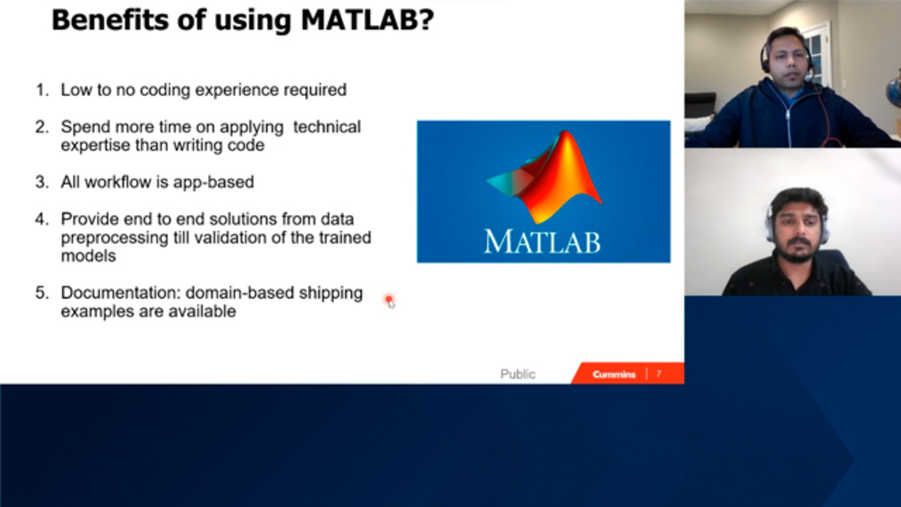
All right. So we used Matlab for our platform for developing these models. There are a lot of benefits that are associated with using Matlab, such as there is low to no coding experience required, so a beginner user can also develop these models with some knowledge of Matlab. Now, what that helps us is we can apply the time to developing these models without specifically spending a lot of time on writing codes. So we can get more out of the platform without having to spend a lot of time on the code development work.

All the workflow is app based, which allows us to, again, very easily integrate different machine learning models to be able to utilize them for our engine simulations. It also provides an end to end solution from data preprocessing till the validation of the model. So basically starting from integrating the data that we have from the engine into these tools, processing that data, making them work for development of the machine learning model, and then applying it for validation of these models.

So all that framework is available as an end to end solution. And finally, the documentation. So it comes with a very significant amount of documentation that helps people build these models easily by following those documentations. Also comes with a lot of examples that people can utilize for these purposes. So with that, I will hand it over to my colleague Britant to talk about the methodology.

Thank you, Shakti. Hi, myself, Britant Sureka. So I'll be taking over from now where firstly I'll be talking about the methodology. Now firstly, this methodology was adopted to build LSTM based deep neural network models where a detailed approach was taken to also optimize the associated hyperparameters.

Now in this methodology, as a first step, what we do is we define the neural network architecture. In this step, we define how many layers do we want, what type of layers do we want. Do we want to introduce LSTM layers into our model? What kind of activation functions do we want between the layers? And also, how many neurons we want for each layer. So in this step, we basically define the skeleton or the architecture of the deep neural network model.

Once we define that, then we go to the second step where we define some initial values of the hyperparameters So as per the architecture defined, we will be having some parameters such as learning rate, number of training iterations, solver options, software options, and other hyperparameters. So in step number two we define some initial values to those hyperparameters, and then we move on to the third step where we start training the model for a particular response.

At the end of step three we get the prediction from our trained neural network model or trained deep neural network model. And based on the results we then move to step four, where we firstly try to optimize the parameters that we have initially defined in step number two. So we try to optimize some parameters, such as learning rate, number of training iterations, software options, solver options.

At the end of step four, If we still don't get an acceptable accuracy or satisfactory result, then we have to go back to step number one where we try to, again, optimize the architecture itself. Suppose, do we want to introduce multiple LSTM layers or do we want to change or add a particular activation function? Do we want to increase the number of layers or the number of neurons?

So I would say step number one through four is an iterative process where we keep optimizing the architecture and the associated hyperparameters until we get to a satisfactory result. Once we get a satisfactory result, then we move to step number five through six where we are trying to optimize the process by generating the code of the manual work that was done from step one through four, and then implementing the code for other responses. So this was the brief idea about the methodology that we have taken to build LSTM based deep neural network models.

Now, let's move on to the results. In this slide, I'm firstly showing the results of a traditional feedforward neural network model where the only optimization that was done was number of layers and number of neurons in each layer. These are not the LSTM based deep neural network models, which we have just discussed in the methodology slide.

With this traditional approach of developing neural network models, the observation was that for parameters such as exhaust temperature, we had an error-- we observed an error of around 10%, which is not acceptable for our application. But for other parameters, such as exhaust flow, that can be seen on the right hand side, we were able to get good accuracies and prediction accuracies within the acceptable range of our application.

Now with this observation, this was a motivation for us to do a detailed analysis and follow the methodology that we just looked into for improving temperature predictions, which we were lacking in a traditional feedforward neural network model. Moving on to the results of the detailed approach. The left hand side plot is the same plot from the previous slide where we used a traditional neural network model and observed an inaccuracy of 10%.

When we introduced LSTM layers and other activation functions and optimized the hyperparameters in a very detailed way, we were able to reduce the error from 10% to 1%. And this is an acceptable error band for our application. This was for exhaust temperature, and we observed a similar story when we used another temperature prediction but sense that the different location of the engine, which is at the inlet of the aftercooler.

This is, again, a temperature prediction, and on the left hand side we see the results from a traditional feedforward neural network model where initially the error was 5%, even after optimizing the number of layers in neurons, and with an R square value of 0.85. But when we took a detailed approach of developing the models by introducing LSTM layers, we were able to reduce the error from 5% to 2%, and this is within the acceptable range of our application.

This is the results slide of all the critical parameters that we wanted these models to predict, and what we can see is that for all the parameters such as exhaust flow, turbo speed, exhaust temperature, peak cylinder pressure, brake torque, and in engine out nox, which is emission, we were able to build models that has R square value equal to or greater than 0.95, and correspondingly, very low NRMSE values. So we were able to build models which are able to predict decently for all the parameters.

To summarize, machine learning models were developed to predict various engine performance and emissions. And through the approaches that we have taken, we were able to build models with prediction accuracies of 0.95 and above for all the responses that we want. We took two approaches of developing machine learning model.

The first approach is the traditional feedforward neural network model, which gave us good accuracies on pressure flows and emissions but were lacking in temperature prediction. With this kind of neural network models, we had a factor of real time of one by 1,500 for predicting 26 responses in series. So this model gave us results almost instantaneously.

The second approach and the motivation for the second approach was improving temperature predictions, in which we have taken a detailed approach of building machine learning models by introducing multiple LSTM layers, different kinds of activation functions, and also optimizing the hyperparameters in a very detailed way. We were able to improve the temperature predictions of the machine learning model and come within the acceptable range.

These models are comparatively heavier or computationally a little expensive than the first approach, which is a traditional neural network model, and we had a factor of real time of around 1 by 800 for predicting 26 responses in series. Even though this is slightly-- this is slower than the first approach, but this is still very fast compared to factor of real time, and serves our application to the best. So with both of these approaches, we were not really able to build models within acceptable prediction accurations, but also had a factor of real time much faster than real world and serves our application to the best.

To summarize, machine learning models provides us the opportunity to optimize and control engine performance and emissions and with the luxury of easy deployment capability. Finally, I would like to acknowledge all my team members and support from MathWorks, Koustubh, and Dr. Rishu, who have been instrumental in the success of this talk. With that, I would like to thank you and open for questions.