Real-Time Motion Planning for Collaborative Robot Arms
From the series: MathWorks Research Summit
Changliu Liu, Carnegie Mellon University
Human-robot interactions have been recognized to be a key element of future robots in many application domains such as manufacturing, transportation, and service. For example, various collaborative robots are cooperating with human workers in factories. It is challenging to design the behavior of those co-robots. The design objective is to ensure their behavior is both efficient and safe. In a well-defined, deterministic environment, these requirements have already been achieved by state-of-the-art systems. However, interactions with other intelligent entities bring large uncertainties to such systems. Moreover, onboard computation power is usually limited to account for all possible scenarios. These represent the major challenges faced by co-robots. The problem that this talk is trying to address is how to design the behavior of those robots in dynamic, uncertain environments under limited computation capacity in order to maximize efficiency while guaranteeing safety.
This talk mainly addresses the problem from a motion planning perspective. In order for the robot to be responsive to environmental changes, it is critical that the motion planning algorithms run in real time. Moreover, the planned trajectory needs to be both collision-free and time-optimal. However, the nonconvexity of the motion planning problem makes computation expensive. Liu et al. developed the convex feasible set algorithm (CFS), which is an efficient nonconvex optimization solver that can be applied to both the trajectory planning problem and the temporal optimization problem. Experiments on different problems show that the CFS algorithm is more efficient than other state-of-the-art nonconvex optimization algorithms such as sequential quadratic programming and interior point method. With the CFS algorithm, the collaborative robots can generate trajectories in real time, and are thus more responsive, safe, and efficient.
The CFS algorithm transforms a nonconvex optimization problem into a sequence of convex sub-problems by constraining the original problem in a sequence of convex feasible sets. It is efficient because the unique geometric structure of the problem is efficiently exploited by relaxation and convexification. One consequence was that the step size of the algorithm was unconstrained, hence the number of iterations was greatly reduced. Another consequence was that line search in CFS was not needed, hence the computation time during each iteration also decreased. Most importantly, as the feasible set was directly searched, the solution was good enough even before convergence. “Good enough” meant feasible and safe. Hence, the iteration was safely stopped before convergence and the suboptimal trajectory was executed.
Published: 17 Mar 2023
Thank you. It's my great pleasure to be here sharing with you about our research on real-time motion planning for collaborative robots. So collaborative robots actually appear in many application domains and in today's talk, we mainly focus on industrial collaborative robot arms as shown in the first case. It is challenging to design the behaviors of those co-robots. The design objective is for those robots to be both efficient in finishing various tasks and also stay safe, both safe to yourself and safe to other human users.
In a well-defined and deterministic environment these requirements have actually been achieved by the state of the art. However, it's the interactions with other intelligent entities, especially humans bring a lot of uncertainties to the system and in a lot of case the onboard computation power is usually limited in order to account for all the possible scenarios.
And these two represent the major challenges faced by the co-robots. The research problem that we are trying to solve is, how can we design the behavior of those co-robots in dynamic uncertain environments and their limited computational capacity in order to maximize their efficiency while still guarantee safety?
In today's talk, we will mainly deal with the motion planning part of the behavior design, which we formulate as an optimization problem has shown there. So the cost function is for task performance and motion efficiency where we optimize a function that depends on the robot state, the robot input and the robot goal. There are a lot of constraints on the system. The first kind of constraint is the dynamic and feasibility constraint, which is represented by a set of constraint on control and the state, as well as ODE constraints on the system dynamics.
The last constraint is the most important constraint, which is the safety constraint during interactions, which is defined as a set constraint on the robot state and the set depends on the human state.
So typically, the safety constraint is defined as a collection of states, such that the minimum distance between the human and the robot is greater than a threshold. And in order to facilitate faster computation, the geometries are simplified to capsule representations as shown in the figure there. And the radius of the capsule is a design parameter, such that the vulnerable part of human body has large radius-- for example, the head.
And the safety constraint is actually very hard to deal with doing real time computation because the human dynamics is unknown to the robot and we have sensor noise and so then we do not have very clear measurement of human state. In order to deal with this kind of difficulties, we actually need real time motion planning and replanning in order to handle those uncertainties and be responsive to the change of the environment.
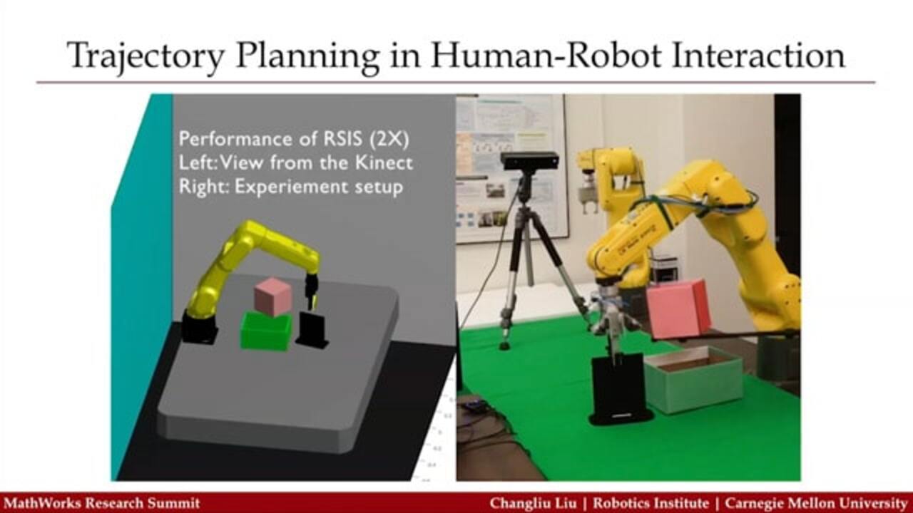
So this video is to illustrate how real time motion planning can facilitate human-robot interaction. The left part of this video is showing the perceived environment by the robot through the connect over behind the robot as you can see in the real video there. The trajectory is the planned trajectory. Although we plan in the joint space, but for illustration we just show the trajectory for the end point.
So the robot trajectory is actually updated from time to time in order to respond to the change of the environment and in order to ensure this kind of behavior we actually need very fast motion planning. And for this experiment everything is running MATLAB.
So how can we make sure that we can solve the optimization problem very efficiently online? So in order to take advantage of numerical methods we actually discretize continuous time optimal control problem into a discrete time motion planning problem by just sampling the trajectories and then the optimization just is turned into general non convex optimization as shown in the bottom problem there.
Usually, this kind of non convex optimization problem is solved using sequential quadratic programming, which iteratively solve a quadratic sub problem and the quadratic sub problem is obtained by quadratic approximation after Lagrangian of the original problem and the linearization of other constraints.
However, it is very hard for SQP to be in real time because it is a generic algorithm and it lacks the unique geometric structures of the motion planning problems that we are facing.
And what are the geometric structures of the problem that we're solving? They're actually two structures or two features. The first feature is that we have symmetry in the control input, both in the cost function and in the constraint. And the second feature is that we have a fine dynamics. That means the control input, u, does not enter the nonlinearity part of the equality constraint.
And with this understanding we can illustrate the geometry of the problem in a very simple 3D space where the horizontal plane is the space spent by the trajectory of the state and the vertical axis is the space spent by the trajectory of control input.
So the nonlinear equality constraint actually defines a nonlinear manifold in this space. There are several holes taken out of this manifold due to the state space constraint, gamma, and the holes are complements to the gamma. The contours of the cost function is shown on the manifold there.
Although the cost function itself is usually designed to be convex, the contours on the manifold is non convex since the manifold is nonlinear so it is very hard to search for a solution on this nonlinear manifold with a lot of holes. But as the problem is symmetric and affine. So what if we look for solutions in the volume above this manifold? Like the manifold, there is a linear structure in this new search space and the cost function is convex in this new search space.
And the best thing for this new search space is that, due to symmetry in the cost function the cost goes down if we move along the negative direction of the u axis assuming the horizontal plane is where you achieve zero.
So the optimal solution always lies in the bottom of this volume. That is, if we run optimization algorithm for example, gradient descent, the mechanism will automatically pull the solution down to the bottom of this value where the non linear equality constraint is automatically satisfied. And to further speed up the computation, the problem can be also transformed to a convex optimization by confining the domain to a convex feasible set of the non convex domain.
And to reduce the error of this convexification we can do iterations. And here we will show how we use iterations to minimize the approximation error. Now we are considering this relaxed problem where the decision variable is reduced to only x and in this relaxed problem the cost function is convex and the domain is non convex.
So for our reference trajectory we just compute our convex feasible set in non convex domain and solve the optimization in the convex feasible set. And this step is very easy because we just call the quadratic programming in MATLAB to compute a solution and then we check if the solution converge or not. If not, we go back. If it converge then we output a solution.
So in a trajectory space this kind of iteration goes like, we first have a reference and then we compute a convex feasible set represented as this red polygon. So the gray part are the infeasible part. Then through this iteration the algorithm will automatically find the optimal in the original problem. Even if we have an initial reference, as long as we can find a convex feasible set for this initial infeasible reference the same process can go through and we can finally find the optimal solution.
So this is actually in the trajectory space, so each point in the space represents a trajectory. In the Cartesian space the iteration goes like, we first-- There is no mouse. So we first have a reference trajectory represented by the dashed line and the algorithm will actually perturb this trajectory, first to the pink one and then gradually converge to the dark trajectory, which is optimal and collision free. And we have shown that this algorithm has guaranteed convergence and optimality and everything we talked here has been implemented in MATLAB.
There are many similarities to this kind of approach. For example, people are using convex corridor or convex tubes to confine feasible area for a trajectory. The idea is to find a bubble for each point along a trajectory and then perturb the trajectory inside the corridor formed by this kind of bubbles. If we shown the convex feasible set in our algorithm in a time augmented trajectory space for a linear system it is also a tube as shown in the blue area there.
However, the key difference between our method and the existing method is that our reference can be infeasible and the convex corridor in our case is maximum in the sense that the convex feasible set are projected to each time set is the largest set in minimum measure. And there are theoretical guarantees that we have convergence to at least a local optimal where for other approaches this technique is used as heuristics. Finally, our method can be regarded as a non convex optimization solver, which can be applied to other problems that satisfy this geometric feature.
We have compared this CFS method with SQP in MATLAB. So the SQP implemented in MATLAB and here's a comparison result. So for this task, we require this robot to go through the four corner points of this square. So in the animation here, path 1, 2, 5 is collision free so there's not many difference between the two algorithm, but path 3 and 4 is initially infeasible and CFS took fewer iterations and compute faster in getting a collision free trajectory. Yeah, the final trajectory looks like this.
But people may argue that SQP is known to be kind of slow in computing non convex optimizations so we also compared our algorithm with Knitro point. But this comparison is done in C++. So as shown in this figure, when the scale of the problem is small. Knitro point actually has comparable performance with CFS, but CFS scales better to larger problems. So that's the algorithm for general motion planning.
In certain cases the path for a robot is fixed so the robot can only resort to temporal maneuvers to respond to emergencies. So sometimes trajectory planning is decoupled, two steps. First step is path planning. Second step is speed profile planning. And speed profile planning for a given path can be posed as a temporal optimization problem. We will use an animation to show how this problem can be solved using temporal optimization.
So suppose we have a trajectory and the horizontal axis represents a time, then we can sample this trajectory in time and given these samples we can find optimal timestamps for those samples which both satisfy the dynamic feasibility constraints but also minimize the total cycle time.
And we can show that if we post a problem as this way the geometric structure of the problem still satisfy the requirement of CFS algorithm. For the sake of time, we are not going to show the details of the derivation, but if you're interested you can look through our papers.
So because the geometric features satisfy the requirements we can still use CFS to solve the problem. So here is some experiment result of temporal optimization on the previous example. Before temporary optimization the robot motion is kind of slow, but after the temporary optimization we can ensure that the robot motion be efficient but still satisfy all the physical constraints.
Here are two tables showing the computation time for both trajectory planning and temporal optimization, as well as the final execution cycle time. So we can see for the temporal optimization does not add too much overhead in terms of computation time but it successfully reduced the cycle time of the robot by more than 50%. OK.
So as a conclusion, why does CFS algorithm gain such efficiency over the others? That is because we explicitly explore the geometric structures of the problem by relaxation and the convexification. So one consequence of exploring the geometric structure is that we do not need to constrain the step size of our problem so the number of iterations is greatly reduced.
And another consequence is that we don't need to do line search anymore so the computation time during each iteration is also decreased. And most importantly, we can directly search in the feasible area so the solution is actually good enough, even before convergence. And good enough means the trajectory is feasible and safe, can be executed. So we can safely stop the iteration before convergence and execute a sub optimal trajectory if time is really limited. So all our codes are available on GitHub and feel free to check them out. Thank you so much.
[APPLAUSE]


Seleccione un país/idioma
Seleccione un país/idioma para obtener contenido traducido, si está disponible, y ver eventos y ofertas de productos y servicios locales. Según su ubicación geográfica, recomendamos que seleccione: United States.
También puede seleccionar uno de estos países/idiomas:
América
- América Latina (Español)
- Canada (English)
- United States (English)
Europa
- Belgium (English)
- Denmark (English)
- Deutschland (Deutsch)
- España (Español)
- Finland (English)
- France (Français)
- Ireland (English)
- Italia (Italiano)
- Luxembourg (English)
- Netherlands (English)
- Norway (English)
- Österreich (Deutsch)
- Portugal (English)
- Sweden (English)
- Switzerland
- United Kingdom (English)