
Simulating Autonomous Flight Scenarios
Overview
As usage of UAV and aerial vehicle applications accelerates, autonomous flight technologies are being embraced to increase efficiency in operations and lower the burden on operators. Developing autonomous aerial systems require ensuring safety and reliability in the broad array of environments and conditions the system will be utilized.
Autonomous UAV scenarios encompass a variety of mission profiles through various scenes while understanding and adapting to surrounding obstacles. Simulation using realistic UAV scenarios and sensor models is critical prior to hardware flight testing and allows engineers and researchers to evaluate autonomous UAV algorithms efficiently while lowering risk.
Attend this session if you are developing or researching autonomous UAV and are interested in how scenario simulations can help evaluate your autonomous flight algorithms.
Highlights
In this session you will learn about workflows to design, simulate, and visualize autonomous aerial scenarios through closed-loop simulations using MATLAB and Simulink with tools provided by UAV Toolbox, including:
- Authoring UAV scenarios with the UAV Scenario Design to define vehicle platforms, sensors, trajectories, and obstacles
- Execute scenario simulations to generate sensor data and test controllers and autonomous algorithms
- Unreal Engine co-simulation to generate synthetic sensor data and to test perception-in-the-loop systems
- Customizing UAV vehicle meshes and scenes for specific flight applications
- Multi-UAV scenarios to simulate and test swarm algorithms
About the Presenters
Fred Noto – Robotics and Autonomous Systems Industry Manager
Fred Noto is a Robotics and Autonomous Systems Industry Manager at MathWorks Japan where he works with robotics and autonomous systems customers to realize solutions for complex and advanced robotics systems development. Prior to joining MathWorks, Fred worked at Northrop Grumman in Los Angeles, and as a Guidance, Navigation & Controls Engineer, he gained experience working on autonomous algorithms and controls systems for ground and aerial autonomous systems.
Naga Pemmaraju - Product Manager - Robotics and Autonomous Systems
Naga Pemmaraju is a Product Manager in Robotics and Autonomous Systems at MathWorks, Hyderabad. He focuses on reference applications and ASAM standards for Autonomous Systems. Prior to this role, he worked as Application Engineer at MathWorks in helping customers adopt Model-Based Design approach. He also worked as controls engineer at Caterpillar, Northern Power and Vestas Wind Systems.
Recorded: 28 Jun 2022
Hello, and welcome to this webinar on Simulating Autonomous Flight Scenarios. My name is Fred Noto. I'm an industry manager for robotics and autonomous systems. And presenting with me will be Naga Pemmaraju, product manager for robotics and autonomous systems. In this presentation, we'll cover how MATLAB and Simulink can be used to define simulation scenarios to virtually test your autonomous flight applications for aerial systems so that you have confidence that your autonomous aero systems perform as expected-- reliably and safely.
Now before we dive into the content, allow us to introduce ourselves a bit more. Again my name is Fred Noto. I've been with MathWorks for almost 10 years in MathWorks Japan. And I've been enjoying helping MATLAB and Simulink users build their advanced systems and working together to address the development process challenges. My background is in the aerospace and defense sector.
And I've had the pleasure to develop autonomous mobile and aerial systems. For autonomous aerial systems, I've been involved with flight controls and GNC, aerodynamics, unmanned autonomous systems development, and mission planning software to name a few areas. Modeling and simulation have been a large part of my career. And I've also been lucky to be involved with projects from design to flight testing. So I've felt firsthand how important virtual testing can be. Enough about myself. Naga, can you introduce yourself as well?
Sure, Fred. Hello, everyone. I'm Naga Pemmaraju, product manager in the robotics and autonomous systems. I'm based off MathWorks in the office. And I'm with MathWorks for over seven years now, mainly supporting customers in model-based design workflow adoption.
My experience in autonomous systems include working on unmanned aerial vehicles, supporting customers for autonomous underwater vehicles and also autonomous guided vehicles. Thank you. Back to you Fred.
Thanks, Naga. So let's get into the content. Here we have the agenda for today's webinar. We'll start with the introduction and then get into the technical topics, the first one being designing autonomous flight scenarios using MATLAB and Simulink. We'll move on to evaluating autonomous algorithms through scenario simulations and then get into increasing scenario simulation fidelity with 3D simulators. Then finally, we'll summarize the content and provide a few key takeaways.
Let's get started with the introduction. Now I'm sure you all see the increase in the usage of aerial systems for a broad range of applications. Aerial systems are being used for media, delivery and transport, inspections, agriculture and construction tasks, and others as well.
Traditionally, these aerial systems are controlled by an expert pilot remotely controlling the system. However, with the promise of aerial systems to make work and our lives more efficient and enjoyable, the need for scalable operations of aerosystems is needed for which a solution is autonomous flight. And thus, research and development for autonomous flight is increasing.
Of course, a safe, reliable, and stable platform is a necessity. But the autonomous flight capabilities, which consist of controls, motion planning, and perception also need to be safe and reliable to be accepted for practical use. Now developing a new autonomous flight technology can be challenging.
Of course, there are many challenges involved in developing such autonomous flight applications. A few key challenges highlighted today are, first, the testing of autonomous flight. This is especially true with hardware flight testing, which is always time intensive, costly, and has the risk of crashing and breaking the hardware. You typically want to make sure the autonomous system is in good shape prior to testing on hardware.
Second, in order to understand and prove how the autonomous flight algorithm will behave, a tremendous amount of test cases and flight conditions need to be evaluated. These aerial systems are going to be used in the real world. So safe operations and the situations they may fly in need to be verified.
Third, repeatability of tests is needed. For example, if you find an error in the autonomous software in a specific test case, you would want to verify your fix in the same test case and condition. And this is extremely difficult to do with hardware flight testing. And for virtual testing, you would want deterministic simulations. So these are a few of the challenges that we hope to cover today.
I'm sure everybody understands the importance of simulations when developing aerial systems, especially when they're autonomous. Simulations are necessary to identify and eliminate errors early and helps to verify your autonomous aerial systems even before the hardware is available. Virtual testing is obviously easier to set up than hardware testing, since you would need to define the test cases and parameters for simulation rather than fiddling with hardware setup.
Additionally, this would allow you to reduce the amount of hardware flight testing to the absolutely required test cases. Of course, you need to define your simulation test cases. In addition to the standard flight conditions, you can perform what if scenarios more easily with simulations. For example, in autonomous flight, you may encounter cases of obstacles mid-flight. This is much easier to set up and test in simulation rather than hardware in real flight.
Another example is weather conditions. We can't control the weather yet. So it's much easier to set some parameters to add wind or fog or rain in a simulation. And finally, deterministic simulations are key to ensure your autonomous aerial systems will perform as expected and will be helpful when re-using your test cases for regression testing down the line as well.
Now, there are, of course, many types of simulation and, of course, many supported by MATLAB and Simulink. These range from open-loop simulations where, perhaps, you have just designed an algorithm for autonomy and you want to perform some initial verification or evaluation of this algorithm. As you move forward, you might add additional components to the autonomous algorithms, perhaps including perception and capabilities with Lidars.
In this case, you don't have real data. You want to generate synthetic data through simulations. The initial step for this is cuboid simulations, which would allow you to quickly author scenarios, including the environment, simulate and evaluate your autonomous flight applications while generating sensor data.
As you move on and gain more confidence in your autonomous algorithm, you can move up in fidelity to more photorealistic simulations, in many cases, using gaming engines here. This will allow you to really test your autonomous algorithms with perception in more realistic environments and also test perception algorithms which involve camera visual imagery. In this session, we'll focus on simulations for cuboid and photorealistic environments for closed-loop simulations.
Fred, so I see that simulation is definitely important in the process of developing and evaluating autonomous flight applications. But there seems to be many steps involved to set up these types of simulations. Right?
Well, there is, of course, set up of involved. And in this next section, we'll get into defining the scenarios to assimilate autonomous flight. Let's start by thinking about, what are the basic components needed to simulate autonomous flight? There is, of course, the platform or the aerial system that will be performing the flight to be used in a specific task.
The system will consist of some sensors to be able to localize itself and be aware of its surroundings. There's also the environment in which the aerial system will be operating in. This can include buildings, trees, power lines, or other drones, depending on where the aerial system will operate.
The UAV will then plan and optimize path through the surrounding obstacles. And also, we'll need to adjust the trajectory if unexpected obstacles are encountered. These are the basic components and the overview of scenario elements. With MATLAB and the add-on product UAV Toolbox, you can programmatically define an autonomous flight scenario.
Here's an example of creating a scenario for a UAV by defining the platform, setting waypoints to fly through, adding sensors, an INS sensor in this case, and obstacle meshes to the scene, which will act as stationary building obstacles. I've highlighted a few of the key functions to define the scenario here. And running the script, you can visualize the scenario simulation within MATLAB.
Now this, of course, is a basic scenario simulation to get accustomed to defining scenarios. If the actual location of operations is known and there is data available, you can also import terrain data through digital terrain elevation files or detail. If there are OpenStreetMap, OSM, files available, you can import the building meshes from the file as well, allowing you to quickly define the scene without manual entry.
Now, what about model-based design? You can connect the scenarios with simulation models using the scenario simulation blocks provided by UAV Toolbox. You can, of course, use a guidance model block to define a fixed wing or multi-rotor platform and interface to the scenario using motion, read, and write blocks. There are blocks available to simulate sensors and also read point cloud data from the scenario simulation.
The scenario configuration block links the Simulink simulation to the scenario while the scenario scope block allows for visualization during simulation. Trajectories can be defined in many ways, for example, using the UAV Toolbox blocks for waypoint or orbit follower. And you can even add initial autonomy with the obstacle avoidance block. With these, you can use plant models, trajectories, and autonomous algorithms designed in Simulink in the scenario simulations.
Here's how it looks in an example model of basic obstacle avoidance. In this case, a UAV is modeled using the guidance model block and is provided with a waypoint trajectory and also includes obstacle avoidance as an autonomous algorithm. The blocks on the left are the interfaces to the defined scenarios. In this case, there are pillars defined to block the path of the UAV.
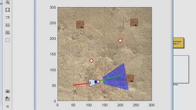
We simulate the model to test how the UAV flies. And you can visualize this simulation here. The green dot is the starting location, and the red dots are waypoint locations to fly through. You can see that this scenario has placed obstacles in the path of the UAV trajectory. As the UAV flies towards the obstacle, the Lidar point clouds are processed to detect an obstacle. And the obstacle avoidance algorithm provides steering commands to avoid collisions.
And if you have tunable parameters in Simulink, for example, we have a sliding bar at the top to adjust the look ahead distance for our obstacle avoidance algorithm, you can change the parameters and resimulate to view the changes here. In this case, increasing the lookahead distance seems to result in a smoother trajectory to avoid these pillars in the trajectory path.
We just talked about how you can programmatically define autonomous flight scenarios in MATLAB and sync them with Simulink models. However, defining scenarios programmatically can be cumbersome if you're new to using these tools or aren't accustomed to programming in general. For these cases, UAV Toolbox provides the UAV Scenario Designer app to help easily define autonomous flight scenarios.
This app allows you to interactively build scenarios on the screen by placing objects in the scenario or importing elements, defining trajectories, basically defining or customizing this scenario in general. You can also simulate and visualize the scenario right in the app so that you can verify this is what you want to simulate prior to exporting the scenario to integrate with your autonomous algorithms.
Let's take a deeper dive into how to use the UAV Designer app. You could open the app by going to the Apps tab in MATLAB and selecting UAV Scenario Designer from the list of apps here. You could also enter UAV Scenario Designer into MATLAB's command window. And we'll hit enter. Open up the app here.
And when the app is open, we'll begin by adding some scene object meshes that will be used as building. We'll select polygon, in this case. Select the preloaded object mesh. Hit import. And select an area on the scenario canvas to add the object. You could change this location of this object and the height as needed. We'll set the height here to 30 meters. And we'll also hit the Snap to Ground Elevation button so that the bottom of the scene object aligns with the ground plane.
Now let's add a platform to this scenario. We'll select Quadrotor over here. And again, click an area on the scenario canvas to place the platform. Hit the Zoom to Scenario to zoom in and have a better view of this current scenario. We'll change the position and the color of the platform as well. So you could customize that.
Next, we'll add a Lidar sensor to our quadrotor, selecting the Lidar button. Change the view to the sensor canvas. And then we select the location on the sensor canvas to add our Lidar sensor on or off the platform. You could change the position afterwards where setting the sensor along the y-axis to the quadrotor here.
Now let's go back to our UAV scenario canvas. Next, we'll add a trajectory for our quadrotor to fly. Go to the Trajectory tab, and we clicked the Add Waypoints button. And then you could interactively define the trajectory for this quadrotor fly. We're just going to fly around the building here. And then you can interactively drag and drop the waypoints to move its positions as needed.
You could also adjust the altitude of these waypoints by opening the time altitude plot and interactively moving the altitude of each waypoint up or down. There's also an option to do this in tabular format by-- we'll do this in a second here-- but selecting the Trajectory Table button shows the waypoint details data in tabular format. And you could edit the values here in the table as well.
Now you could zoom in, view, rotate it around to get a better sense of what the trajectory looks like. Finally with this, we could simulate and visualize right in the Scenario Designer app to see how the quadrotor will fly through the specific trajectory. So we'll hit Run here in the scenario view. And you can see the quadrotor fly along its defined trajectory. Let's take another look.
So that's an introduction to how to define a simple scenario using the UAV Scenario Designer app. Now I'm sure defining a whole city scene would take a lot of time manually. So let's take a look at how to import terrain and building mesh data to accelerate scenario creation. Let's start off in MATLAB and first create a scenario at a specific location using the UAV scenario functionality.
Use Add Mesh to import terrain data from DTED files. You could also import building meshes, in this case, where you importing the area around Manhattan from an OSM file. We'll open up the UAV Scenario Designer app. Now that's open. We'll import the scenario that we just defined in the MATLAB workspace. Click on Import Scenario. Select the scenario called Scene that we just defined. And then we let that load.
And we can visualize the scenario in this app. We could see the city block that has been imported. And now, we want to add a platform to the scenario, fixed wing, in this case. We'll click on an area in the canvas. We could, of course, adjust this location. And then let's also add a Lidar to our platform. And then we'll align that along the x-axis of the fixed wing platform here.
Next is to give our fixed wing platform a trajectory of fly through. We'll select the Trajectory tab. Hit Add Waypoints. And then, again, interactively set the waypoints that we want this fixed wing platform to fly through. So we set some waypoints to fly through the buildings. And again, you could open up the time altitude plot to modify the altitude of each waypoint interactively. Again, we're doing this dragging and dropping the altitude of these.
You could also, again, use the trajectory table as needed to see the waypoint data tabular format. So we'll just change some of the locations here. Then let's go and simulate the UAV scenario. Before that, we'll change the update rate and the number of frames. Hit the Simulate button, which leads to the UAV scenario view.
Zoom in a little bit, and then we'll hit Run. And you can see, again, this fixed wing platform flying along the trajectory we just defined in the imported scene of Manhattan. You could zoom in on the fixed wing platform itself to visualize that it is a fixed wing and also its pose as well.
We can move out a little bit to see how this trajectory is flying through the building objects here. So we just saw how we can import terrain and building mesh data to define scenarios, which are more representative of actual environments that the aerial system will fly in.
This UAV Scenario Designer app is great. Fred, can you show us how to use this app with an example use case for testing autonomy?
Happy to do so, and we'll see this in the next section. Here, we'll walk through how to integrate the scenario simulation with Simulink models, which contain the plant model and autonomous algorithms. Let's start by importing a scenario, which we have predefined in the workspace. We can see that this scenario here, Scene, will be loaded. It's a simple city block with some buildings, of course, as we've seen previously.
We could zoom in to get a better view of scene. We could add additional buildings by selecting polygons. Select a mesh from the list, which is predefined. Pick somewhere on the canvas to add that to drag it around to a set position. You can also change the height here. We'll change it to 30 meters. Snap it to the ground elevation. And that's a basic scenario, which we'll export out to MATLAB after customizing it just with an additional building. We'll change the scenario name back to Scene and export it. So that's ready to use.
Now, we'll switch over to the Simulink model, which we're interfacing the scenario to where you're using the scenario simulation blocks here to interface. We can see that the block parameter for the scenario configuration block was pointing to scene. We have the blocks to interface the Lidar, as well as the vehicle itself with the motion read and write blocks. And the scenario scope will allow us to visualize the scenario as it's being simulated.
We also have the autonomous algorithm in the Simulink model. Here, we have a simple obstacle avoidance algorithm through using the obstacle avoidance block from UAV Toolbox. And at the top level of the model, you can also see we have the multirotor UAV plant model to the right. When we simulate this model, we can visualize the UAV flying in this scenario that we've exported. So we have the scenario scope on the right and the Lidar point clouds to the left.
Let's zoom in a little bit to see the multirotor flying through these city buildings. And we could see the changes in the Lidar point cloud as well as the UAV flies through the city. So that was a simple scenario. But let's imagine that we want to customize this scenario to test our autonomous aerial systems in different settings and with different obstacles or test conditions.
Let's modify some of the building positions and locations to make it more difficult for the UAV to navigate around and force our UAV to plan a different path using its obstacle avoidance algorithm. We're going to change three of the building locations so that they're clustered more closely together and change their heights to 60 meters so that the UAV just can't fly over them. The building colors are also changed from green to be more colorful, so we can clearly visualize the modifications during the simulation.
Now let's imagine we want additional obstacle aside from just stationary buildings. And we could do that by adding additional platforms. We're going to select a multirotor, add it to our canvas here, and give it a trajectory to fly. We're going to make it loop around in an open area and come back towards our ego vehicle.
Now the cross-section for a multirotor is very small, and it's a little bit hard to see the detection force. So we're going to add what's called a cuboid platform to our scenario as well. Now we're going to change the geometry of this cuboid platform to be fairly large-- 3 by 3 by 3 meters. Give it a trajectory to fly slowly towards our ego vehicle. Now it's not very realistic, but this is just to show how you could simulate some obstacle and detect these as well in your scenarios.
We'll modify the altitudes for these trajectories to be closer to our ego vehicle so that they'll be viewed as obstacles during the simulation. Once those altitudes are modified, we'll hit the Export Scenario button once again and change it to Scene since that's how we have our model set up. And over in our Simulink model, we could hit Run once again. So click Run, and we can start visualizing the simulation in process.
Again, we'll enlarge these views. Zoom in a little bit to better see these. And right off the bat, I think you can notice that the buildings here have changed in color and both heights, the ones that we've clustered closer together. Also zooming in, so there's the buildings here. Clearly, they're a lot taller than the others.
And you could also see the obstacle platforms that we added. Their trajectories that they've flown through are also colored. They're yellow and purple, in this case. Clearly, one's a large cube. And on the point cloud side, here you could faintly see the obstacle multirotor passing by our ego vehicle. So again, the multirotor cross-section is small, so that is a small detection, but a detection nonetheless.
And then a little bit down the line, you could see the cuboid platform approaching our ego vehicle. So this is a much larger, 3 meters around platform here, which is a cube, again. Not realistic, but it's floating towards our ego vehicle.
And our ego vehicle needs to figure out the path or use the obstacle avoidance to determine a path around this cuboid obstacle, as well as to not collide with the surrounding buildings. And as the ego vehicle passes by this cuboid, you can see that the detection have changed from the front to the back of this cuboid platform, which is an obstacle.
So we've just seen how we could export scenarios from the UAV Scenario Designer app, interface them with Simulink models, which include plant dynamics and autonomous algorithms, and run the closed-loop scenario simulations with a cuboid environment. You could also visualize with scopes how close you got to each of these obstacles, whether they're the obstacle platforms or the buildings. So these are calculations you could do within the Simulink models as well.
So in the previous sections, we walked through how to define autonomous flight scenarios in the UAV Scenario Designer app, export the scenario to interface to Simulink models using scenario simulation blocks, run the integrated simulations, and while simulating, we were able to visualize the Lidar point clouds and the scenario simulations themselves. We also saw how we can customize the scenario, export it again, and run the simulation and saw how the customizations have been applied.
Now this is a powerful first step to evaluate autonomous algorithms, especially for their motion planning and perception algorithms if using Lidar sensors. And this also allows for initial closed-loop simulations with sensor models. Now we just covered defining scenarios and simulating them in cuboid submissions, but there's obviously a gap between the 2.5D cuboid environment and the real world. Naga, can we use more realistic simulation environments as a next step in evaluating autonomy?
Hey. Thanks, Fred. Glad you asked that question. In the next section, we'll cover exactly that. We'll look at simulating scenarios in 3D simulations. We have seen how cuboid simulations are helpful in validating algorithms. As a next step in the development cycle, we test these algorithms with photorealistic 3D simulations. These simulations are really resource intensive and so can be used as a final validation step before testing in actual environment.
So what is the need for high fidelity 3D simulations? One, we want to develop autonomous algorithms and make them learn to adapt for real-world scenarios. For example, you can make a use of these simulations to learn some of the advanced controls like reinforcement learning. We can also use this 3D simulations to test perception and controls in a closed-loop system for different scenes and also visualize motion planning.
We can also generate synthetic sensor data like camera images, for example, not just a visual image but also a depth image or semantic segmentation and also generate high fidelity Lidar data. Let's see how we perform 3D simulations with MATLAB and Simulink.
Here is a shipping example of a UAV package delivery. Let's try to understand the Simulink model. The block we are seeing now is external sensors for Lidar and camera. We have four major blocks here, one for setting up the 3D simulation environment. And then we have a block for the camera model and also one for the Lidar point cloud.
Let's deep dive into these blocks a bit. When we select the simulation 3D scene configuration, we have an option to choose a scene source. Here, it can be a default scene, or we can also select a scene from Unreal and Executable , or it can also be from Unreal Editor. We'll understand a bit more about the Unreal in a later part of this presentation.
We can also select a scene name. Right now, it's a US city block. When you create your own scenes, custom scenes, you can also have the option to select your own scene here. And then we have the scene view what's a Simulink Vehicle.
And here, what you see is basically selecting the weather effects. We can create a rainy atmosphere or a fog. We can also have a cloudy weather. So we can actually simulate such kind of weather scenarios here. So right now, we are just selecting the regular one. We are not selecting any weather effects in this particular case.
Then, let's go to the simulation 3D UAV vehicle. Here, as you can see, we have an option to select the type of the UAV vehicle we want. By default, we have a quadrotor and the fixed wing. We also have an option for custom, like say if you want to build a hexacopter or an octocopter. You have to come up with that.
And then you can actually select the custom option and then choose the right UAV vehicle. And the color, you have an option to choose various colors and then select the right name. And then select the initial translation and rotational values.
Now let's look into the sensor models. First one, the camera module, we have to set the details about the mounting so where exactly we want to mount this particular camera. The mounting location, the relative translation rotational details have to be mentioned under the Mounting tab. What you see here.
Then when we put the parameters, and some of the basic details for the camera are asked here, for example, the focal length, the optical center. What could be the image size and pixels, including the distribution coefficients and then the ground truth, which is very important. One, we get the visual image at the same time. We also can output a depth image or even a semantic segmentation. Such details can also-- we can also get those images from the simulation, which is very helpful for testing advanced algorithms.
Then when we move to the Lidar point cloud sensor block, something similar to the camera, we first need to provide the mounting details. Where exactly this Lidar sensor will be mounted? And similarly, the translational and rotational details. Again, the parameters needs to be provided for the Lidar sensor, like the detection range, range resolution, the vertical field of view resolution, horizontal field of view resolution, et cetera.
Similar to the camera sensor, we also have the ground truth for output location and orientation. So once we have set all these details, the information from the sensors will be provided to the next block, which is on board computer. In this particular case, we are using the same example of obstacle avoidance of what Fred has talked earlier. So we are using the same algorithm. Earlier, Fred was testing this algorithm with the cuboid simulations.
Now we are testing the same algorithm with the photorealistic 3D simulations where the sensor data is coming from the 3D simulations. If you get into the obstacle avoidance, we have the same obstacle avoidance block, which was used earlier. Again, this block ships with the UAV Toolbox, which asks for the basic details like the position, the orientation, the point cloud details, and also the target position. And provides the output as the desired direction, yaw, and status.
And the last one is the actual multirotor where we provide the guidance logic and the dynamics of the UAV. When we look into the inner loop and plant model, again, we have the controls and the guidance logic. And the controls here is basically the position controls, velocity controls, and altitude controls. And coming back to the guidance model, this, I would say, is a low fidelity dynamics what we have considered. Again, this particular block is shipped with the UAV Toolbox.
So this is a reduced-order model what we are considering. Here, we have an option again to select the type of model. It could be a multirotor or a fixed wing. And then of course, the other details like, what should be the data type? And what are the initial states like position, velocity, alorcity angle. Similarly, with respect to the configuration, what could be the yaw rate, thrust, pitch, and roll? So we have to provide some of the basic details here as a part of the guidance model.
Once we configure this, we have a dynamic set in place, and we are ready to perform the simulation. Let's look into the co-simulation with Unreal. We have seen how the model has been set up. When we run the simulation, the model gets compiled first and then initialized.
Now, we should be able to see the simulation in a few moments. There you go. So let me explain what you see on the screen. So first, we see a model on the down, left corner-- the same model what we have just seen. The one above that is basically the camera image that's been sent to the model.
The rightmost corner, top corner is basically the Unreal scene what we are seeing. And the one below that is basically the Lidar point cloud. So as we see the UAV navigating between the buildings, this is US city block what you're seeing here, the scene. So we are seeing the UAV moving between the buildings, and there's a camera mounted on it. And it has its own Lidar mounted on it.
And basically, we are sending the image data and the Lidar data that we see here back to the model. And then we're actually testing our algorithms with this data. So this is the advantage of doing this photorealistic simulations. Typically, it's tough for us to get the vehicle outside and do all of the simulation in the real world. So that's when the photorealistic simulations will be very handy. And now we can see the UAV landing.
So we have seen the camera sensor can be actually mounted on top of the UAV. So it can exclusively send us some kind of visual images, which can be transmitted back to our model. These images help in path planning and object detection algorithms.
It can also provide the depth camera. So the depth image is a grayscale representation of a camera sensor output. So these maps visualize camera images in grayscale where brighter pixels indicates objects that are farther away from the sensor. You can use this depth visualizations to validate depth estimation algorithms of your sensors.
It can also output semantic segmentation. Semantic segmentation provides-- basically, it's a process of associating each pixel of the image with a label such as this is the road, building, traffic sign in the 3D simulation environment. You generate semantic segmentation data according to the label and basically test your classification methodologies. So again, this is one other way of testing your classification schemes using this data.
We can also use Unreal simulation to map an environment using StereoVisual SLAM. Here, what you see is basically they're flying a UAV carrying a stereo camera through a set of waypoints as shown in this particular scene. This is a US city block scene. And again, we are making the UAV fly through a particular set of waypoints. This will help us to generate a map and localize the UAV based on simulated camera images.
This example, what you're seeing on the screen uses Unreal Engine simulation from UAV Toolbox and the visual SLAM algorithm from Computer Vision Toolbox. This is a final map of the path that the UAV took. And here, you can actually visualize the path and the surroundings. And basically, it's trying to map the complete environment.
Next, we want to see how we can test our autonomous flight applications for varying conditions. We have already seen how we can run code simulations with MATLAB and Simulink with Unreal. But now, if you want to test this in varying environmental conditions like a rainy scene or a fog, we can also perform that.
So on the right side, what you're seeing is basically testing the same simulation but in a different environment, which is a rainy condition. Again, we can also do the conditions like foggy weather or even a cloudy weather, et cetera.
We can also customize the 3D simulations. We can have our own custom vehicle measures. For example, if you want to build a hexacopter instead of using a quadcopter or a fixed wing, so we have the functions that help you to build such custom vehicle meshes and then export it into Unreal Engine. So these are some of the functions that we provide out of the box.
We can also help you in building custom scenes. So what you have seen so far is a US city block. So you also want to use a different scene like, in this case, you're flying on a highway or any other scene. And it can be even a suburban scene. So here is a suburban scene with all the houses, and locative. So we can create this scene and see how our UAV flies in this environment.
So let's look at how we can create such kind of scenes. We use RoadRunner as a tool to create such scenes and then export the scene to Unreal. Here is a workflow. We first create the scene in the Roadrunner, and Roadrunner provides a good set of libraries assets for creating the scenes. Then we export the whole scene into Unreal supported format like .fbx or datasmith format.
Then, this will be imported into Unreal. The image, what you see, is in the Unreal environment. Then, we integrate that with MATLAB and Simulink with the supported blocks, like the configuration block, the sensor blocks, et cetera. Let's see this in action.
Here is Roadrunner, a scene we have just added a house and then basically changing the orientation. As you can see, there's a lot of assets available. Using this, we'll be basically creating the scene, exporting it into that aspect format. And once we have that format, we go to Unreal, import the same scene into Unreal. So now, we can see the whole scene in the Unreal Engine. It is a complete scene. And whatever you're seeing the visualization is in the Unreal Editor.
Here, again, we're trying to integrate this with MATLAB and Simulink. In the simulation 3D scene configuration, we're just changing the scene from US city block to the new scene that we just created. And we are using the 3D camera to take the images and basically perform core simulation with Unreal and MATLAB and Simulink.
So here, you can see the UAV flying in the suburban. So like this, we can create our own custom scenes and test our application. Say if you ever want to test my obstacle avoidance for various scenes, this is a good way to test your algorithms virtually in the 3D photorealistic scenarios.
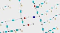
We can also perform multi-agent simulation in the Unreal. Here, you are seeing formation flying, which has multiple UAVs-- one a leader. The three are the followers. We can create such scenes in Unreal and, of course, simulate with MATLAB and Simulink.
So let's summarize what we have seen so far in the 3D simulations. We have seen the blocks that helps us to integrate with MATLAB, Simulink, and perform core simulation with Unreal. We have seen how can we perform mapping and visualization and testing our SLAM algorithms with Unreal. We also seen in how to build our own custom scenes and meshes and then also perform multi-agent simulation. I now handover back to Fred who will walk us through the conclusions and the key takeaways. Thank you very much.
Thanks, Naga. Let's get into the summary. Simulations are a vital part of the development process for aerial systems with autonomous flight. And in this session, we showed how MATLAB is Simulink, along with UAV Toolbox, can help to execute various simulations. Now we focused on the closed-loop simulations with sensor models starting with the cuboid simulations and then moving on to 3D simulations with Unreal Engine.
There are tools such as the UAV Scenario Designer app that makes defining autonomous flight scenarios simple and interactive. We showed different fidelities of simulations. But an important point is to select the appropriate simulation fidelity for your current development phase. Starting with all aspects at the highest fidelity requires computational resources, and, oftentimes, leads to long simulation times.
So an open-loop may be fine for initial algorithm checks, then move on to cuboid simulations for initial closed-loop virtual testing. And when there's more confidence or if testing autonomous systems that include camera sensors is needed, move on to the 3D simulations with Unreal Engine.
So to summarize our key points. Select the appropriate simulation fidelity for the phase you're in now. MATLAB and Simulink can help with these various types of simulations and has tools and apps to ease designing autonomous flight scenarios. And you can integrate these scenarios with your Simulink models containing autonomous algorithms for closed-loop integrated testing of your autonomous aerial systems.
We hope you found what we showed interesting and helpful. And you can try out many of the examples we show today as they're available in the UAV Toolbox documentation. There are also webinars on other aspects of autonomous flight and UAV application development ranging from aerial Lidar processing, flight log analysis, and software in the loop, hardware in the loop, and deployment workflows. Please try out these examples for yourself and check out the other relevant videos. That's it for our session. Thank you very much for your attention.
Related Products
Learn More
Featured Product
UAV Toolbox


Seleccione un país/idioma
Seleccione un país/idioma para obtener contenido traducido, si está disponible, y ver eventos y ofertas de productos y servicios locales. Según su ubicación geográfica, recomendamos que seleccione: United States.
También puede seleccionar uno de estos países/idiomas:
América
- América Latina (Español)
- Canada (English)
- United States (English)
Europa
- Belgium (English)
- Denmark (English)
- Deutschland (Deutsch)
- España (Español)
- Finland (English)
- France (Français)
- Ireland (English)
- Italia (Italiano)
- Luxembourg (English)
- Netherlands (English)
- Norway (English)
- Österreich (Deutsch)
- Portugal (English)
- Sweden (English)
- Switzerland
- United Kingdom (English)