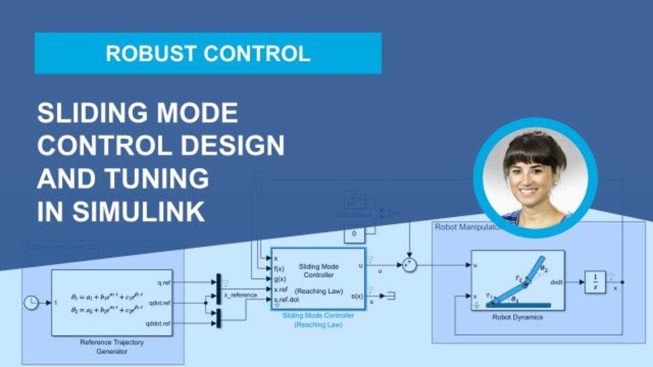
Sliding Mode Control Design for a Robotic Manipulator
Sliding mode control is a robust control technique that ensures precise tracking of desired trajectories, even in the presence of model uncertainties and disturbances. This demonstration includes a quick overview of sliding mode control. It also shows how you can design and tune a sliding mode controller in Simulink® to make a robotic manipulator follow reference trajectories in the presence of model uncertainties and external disturbances.
Click here to check out the example demonstrated in the video.
Published: 26 Dec 2024
In this video, we will show you how to design a sliding mode controller in Simulink for a robotic manipulator. We'll be showcasing the new sliding mode control block that shipped in the 24B release. Sliding mode control is a robust control technique that ensures precise tracking of desired trajectories, even in the presence of model uncertainties and disturbances.
If you're new to this topic, you may want to check out our tech talk, which provides an in-depth explanation of how sliding mode control works along with mathematical insights. We'll focus on practical implementation of sliding mode control in this video. But before that, let's first quickly review the idea behind this control method using a conceptual example.
We'll assume a system with two states, X1 and X2. The state space representation of the system describes how the states evolve over time, where u is input to the system, d is disturbance, and f and g are the system dynamics and input functions.
Here, for simplicity, we're using sliding mode control as a regulator, meaning that we aim to drive the states to zero. But as we'll see later, sliding mode control can also be used for arbitrary reference trajectories. The key feature of sliding mode control is its robustness, even when the system dynamics are not fully known, or when external disturbances are present. To discuss how robustness is achieved in sliding mode control, we will use this phase plane diagram where one state is plotted against the other, along with the time responses for the states and the control input.
When the goal is to drive both states from their initial positions to zero, sliding mode control accomplishes this by first designing a sliding surface and then generating a control action that drives the states towards the surface that is insensitive to disturbances and model uncertainties. Once states reach the surface, they remain on it and slide along it until they reach the desired position. So this process involves a reaching phase and a sliding phase, which are implemented by the controller shown here. We'll explore this further later in the video.
Another notable feature of sliding mode control is its fast execution, as it doesn't require computationally intensive calculations. One drawback of sliding mode control is the chattering in the control input, caused by the discontinuous control action used to keep the system on the sliding surface. While this provides robustness, chattering is undesirable as it can cause actuator damage and unwanted system dynamics.
Sliding mode control mitigates chattering by designing a boundary layer around the sliding surface. Within this boundary, a continuous control action can be used, which prevents the system from bouncing back and forth around the surface. After this quick overview, let's see sliding mode control in action. In this example, we will design a controller for a two-armed robotic manipulator to make its joints follow some predefined reference trajectories.
Here's a Simulink model we will use to design such control system. It currently includes the subsystems but lacks the controller for which we will use the sliding mode control block. But before that, let's see what these subsystems implement. The robot dynamics subsystem implements the state-space representation of the two-armed robotic manipulator, which has four states, joint angles, and velocities controlled by the torques applied at the joints.
Here, f of x and g of x are system dynamics and input functions which depend on system parameters like masses, link lengths, and moments of inertia. These physical parameters of the system are specified in the block dialog of the subsystem. In practice, we never have perfect knowledge of the nominal plant parameters, leading to model uncertainties, but sliding mode control can handle such uncertainties. Here we use the subsystem to evaluate f of x and g of x functions required by the sliding mode controller at runtime. As we'll demonstrate later, we can test the robustness of our controller by specifying system parameters different from those used in the robot dynamics subsystem.
Finally, this subsystem generates reference trajectories for joint angles and velocities defined by the time-varying exponential functions, as illustrated in these plots. Now that what these subsystems implement, let's add the sliding mode control block which is available with Simulink control design. We'll follow this workflow to demonstrate control design, closed loop simulations with the designed controller, and code generation for deployment.
First step in designing the sliding mode controller is to specify system dynamics. Initially, we'll assume perfect knowledge of system dynamics. Therefore, in this subsystem, we set system parameters to match those of the robot dynamics using this code. Remaining steps can be configured using the two different tabs in the sliding mode control block.
Let's start with designing the sliding surface. The sliding surface defines the desired system behavior once the states reach the surface. The dynamics of the sliding surface are represented by a switching function, s of x, which is a linear combination of the states.
When it's 0, the system is on the sliding surface. In our example, we want to drive all four states to their reference trajectories, so we'll use the tracking mode option. This updates the switching function-- hence the control law accordingly to achieve zero tracking error. The coefficients of the C+ matrix determine the characteristics of the sliding surface-- hence the convergence of the tracking error to zero. Once the sliding surface is reached.
Initially, we specify these coefficients to give a slope of minus 1. Feel free to pause the video to go through the math showing how we compute the slope. Before we move to the next step to define the reaching law, we enable the option to use externally sourced derivatives. This adds new inputs to the block, allowing us to provide reference derivatives computed by the reference trajectory generator. By incorporating these derivatives, the controller can enhance performance through additional feedforward compensation. We also put the switching functions to observe when the sliding surface is reached.
Under the second tab, we formulate the reaching law by specifying the convergence rate, selecting a boundary layer, and then configuring associated parameters for each. While these parameters determine how fast the system will reach the sliding surface, the boundary layer ensures that the states remain close to the sliding surface. Initially, we'll use the default settings, which are constant rate and sine functions. And we'll specify the reaching rate.
Now that we're done with the design of sliding mode control parameters, we can connect our controller like this and simulate our model to analyze performance of the designed controller. Note that initially, we'll test the controller without model uncertainties and disturbances. After running the simulation, we can examine the results.
In the top four plots, we see the joint angles and velocities in blue and their reference trajectories in orange. Next two plots show the control inputs, which are the applied torques at the first and second joints. And the last two plots show the switching function outputs.
Let's first discuss the results associated with the first joint only, where we'll also use the phase plane diagram, displaying the error trajectory of the angle against error trajectory of the velocity. For sliding mode control to work as intended, we need to make sure the sliding surface is reached. As discussed earlier, the switching function equals zero at the sliding surface.
So from the last plot, we see that this happens at 0.25 seconds, corresponding to this location on the phase plane. Until this timestamp, the system is in the reaching phase. Once the sliding surface is reached, the system transitions to sliding phase, during which the control input exhibits chatter, due to the sine function to derive both states to their reference trajectories. This is also visible on the phase plane diagram. When we zoom in, we see how the controller forces the system to move along the surface by bouncing it back and forth until the error trajectories reach zero.
If we now look at the plots associated with the second joint, we see that the sliding surface is reached at around 1.6 seconds. From this point on, it takes approximately five seconds to reach the reference trajectories. Here's the phase plane showing the error trajectories for the second joint.
Next, let's explore if we can achieve faster responses by redesigning the sliding surface to have a steeper slope. To simulate this, we choose larger values in these coefficients of the C matrix. We then simulate again.
Before we discuss the results, Here's, the phase plane diagrams for the previous and current simulations where we can clearly see the steeper slope of the sliding surface in the current simulation. Let's see what impact this has on the system responses. To be able to compare results from both runs, we'll show the previous simulation results in yellow on the first four plots.
For the first joint, we observe slightly faster tracking in the angle and velocity responses. From looking at the response plots for the second joint, you may think that the steeper slope didn't result in faster tracking, since it still takes around 6.5 seconds to drive the states to the reference trajectories. But recall from earlier that the sliding surface has an effect on the desired behavior of the system after it reaches the sliding surface.
So with that in mind, this is a timestamp that the system reaches the sliding surface, and we see that it only takes approximately 1.5 seconds for the joint velocity to converge to the reference, as opposed to 4.5 seconds in the previous simulation. However, the overall response is still slow, since now the reaching phase takes much longer than before. And we still have significant chattering in the control inputs.
To fix these, we'll go back to the controller block and, under the Reaching Load tab, change the convergence rate from constant to exponential. This adds an additional control term, which has the effect of increasing control effort to provide a more aggressive convergence when the state deviation is significant. And to address chatter, we'll use the saturation function for the boundary layer and then set the parameters.
Note that we're using the default value for parameter phi, which defines the boundary layer thickness. We simulate and then compare results to the previous run as before. From the first four plots, we observe that the reference tracking has significantly improved for both joint angles and velocities. The exponential rate enabled much faster convergence to the sliding surface, hence the improved responses. We also see that we were able to mitigate chatter in the control inputs by using the saturation function.
Now that we have relatively good tracking and addressed chatter, let's introduce some model uncertainty using this code, which sets the values of system parameters of the subsystem different from those specified in the robotic manipulator. To test the robustness of the controller against this uncertainty, we'll simulate and look at the results.
We see that the controller still achieves good reference tracking even in the presence of model uncertainties. You can further tune the controller parameters to improve performance. For example, selecting a larger reaching rate can achieve faster convergence, as now can be observed from the response plot for the first joint. But this comes at the expense of increased control effort. So there are similar trade-offs that you should consider when designing sliding mode controllers.
Similarly, we can also test the controller performance against external disturbances, which will simulate here with this white noise block. In the simulation results, we clearly see how the disturbance affects the control input signals. We also observe that the controller maintains good reference tracking performance even when external disturbances are present.
Lastly, once you're done with control design and testing, you can generate code for deployment by right clicking on the sliding mode control block, selecting CC++ code, and building the subsystem. Once code is generated, you can view it in the code generation report.
In this video, we designed a sliding mode controller for a robotic manipulator to follow predefined trajectories and discussed the effect of different sliding mode control parameters on the tracking performance, even in the presence of model uncertainties and external disturbances. If you want to explore this example, click the link provided in the video description. This concludes the video.

Featured Product
Simulink Control Design
Up Next:


Related Videos:


Seleccione un país/idioma
Seleccione un país/idioma para obtener contenido traducido, si está disponible, y ver eventos y ofertas de productos y servicios locales. Según su ubicación geográfica, recomendamos que seleccione: United States.
También puede seleccionar uno de estos países/idiomas:
América
- América Latina (Español)
- Canada (English)
- United States (English)
Europa
- Belgium (English)
- Denmark (English)
- Deutschland (Deutsch)
- España (Español)
- Finland (English)
- France (Français)
- Ireland (English)
- Italia (Italiano)
- Luxembourg (English)
- Netherlands (English)
- Norway (English)
- Österreich (Deutsch)
- Portugal (English)
- Sweden (English)
- Switzerland
- United Kingdom (English)