Nonlinear System Identification | System Identification, Part 3

In the last video, we took input and output data from a system with unknown dynamics, and we fit a linear model to it. And linear models are great because there's so much we can do with them. However, sometimes our system is so non-linear that a linear model just can't capture the essential dynamics. And in those cases, we have to fit a nonlinear model.

Now, when you look at nonlinear system identification, you'll quickly realize that there is a web of near infinite options to choose from. We can choose from a ton of different nonlinear model structures, and different model orders, and different optimization algorithms in different parameters, and the list just goes on and on.

And I'm bringing this up because I want to stress that there isn't a simple recipe that you can follow for nonlinear system identification. Often, finding the right model and the right parameters comes down to having some understanding of the system you're trying to model, along with a healthy amount of trial and error. And so in this video, I'm going to take one path through this web of options.

Specifically, we're going to focus on a nonlinear ARX model, but by no means is this the best way or the only way. I'm hoping that in this video you get an appreciation for what nonlinear system identification is, and it sets you on the right path for discovering the best approach for your particular problem. I hope you stick around for it.

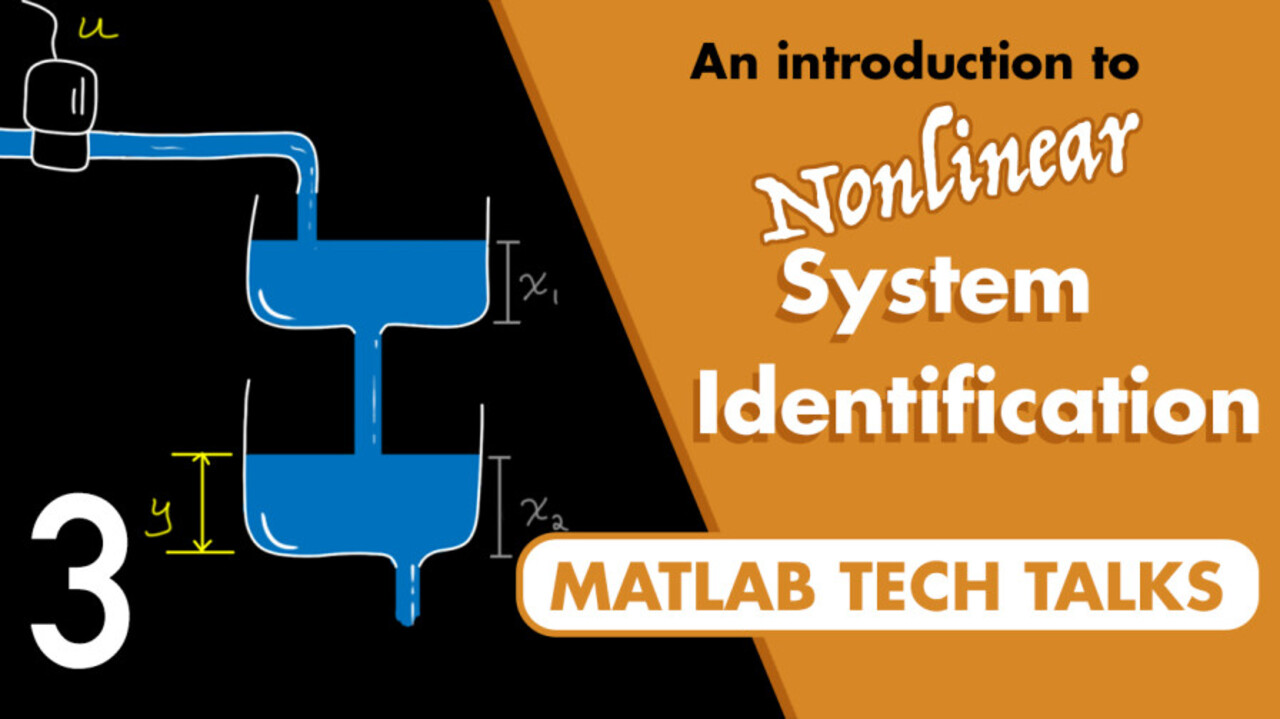
I'm Brian, and welcome to a MATLAB Tech Talk. To begin, let's briefly describe the system that we're going to try to fit a model to. This is a two-tank system. The input into the system, u1, is the voltage that is applied to a pump, which adjusts the flow of water into the upper tank. There's a hole in the upper tank which water flows through into the lower tank, which itself has a hole that drains the water out of the system.

And the output of this system is the height of the water in the lower tank, y1. Therefore, we want a model that takes voltages input and predicts the bottom tank water height over time. And this is fundamentally a nonlinear problem. However, since this is a system identification video and not a physical modeling video, we're going to use data to develop this model.

And I have two data sets from this system. The first is the data that we're going to use to estimate the model. And the second is the data we'll use to validate the model. All right, so first off, if we didn't know anything about the physical system, this data kind of looks like it might be from a linear system or near linear.

I mean, when the voltage goes high, the water level increases and asymptotically reaches some steady-state value. And then when the voltage decreases, the water height also decreases nicely. So it might be worthwhile to first try to fit a linear model to this data.

In the last video, we covered linear system identification, and we fit a differential equation in the form of a continuous domain, first-order process model plus delay term. However, here I'm going to choose a linear discrete time difference equation in the following form. And the reason is because it's going to be a good starting point for our nonlinear model discussion later on. So please just bear with me through all of these numbers.

This is a linear single input, single output ARX model. And by the way, ARX stands for autoregressive plus exogenous inputs, which basically means that the output is a function of past outputs, autoregressive. And it's also a function of the external inputs, or exogenous inputs.

And there's also a possible input delay, and there's this term to model Gaussian errors. And ARX models are a subset of a larger class of polynomial models. And I'm not going to go into detail here, but check out the link in the description for a good write-up on polynomial models.

All right, so using this model, let's say that we want to fit a second order linear equation with no input delay to our data set. So the output is a function of the past two output values and the current input value in the past two inputs.

However, instead of keeping it in this form, we can rewrite it like this in two distinct parts. And this is a good way to view it because we can now clearly see that there is a set of terms that we call regressors that are then scaled by this weighting matrix. In this way, the entire model is simply a linear combination of these regressors, or a linear combination of the past inputs and outputs.

OK, so now let's put this two-part equation into block diagram form, where we get the input and the output both into this block to create the regressor vector. And then that feeds into the linear output function, or the linear combination of those regressors, and the product of those produced the predicted output. And this is our linear ARX model.

So this model seems easy enough so far. However, if we go back and look at our data, we'll notice, again, that the tank height initially starts at about 0.1 meters. And linear models can't handle this kind of offset, since adding a constant breaks homogeneity and superposition principles, which are both requirements for linear systems.

Therefore, we need to do something about it. And one thing we can do is just pre-process the data to remove the offset from the output, then fit a linear model to that pre-processed data, and then add that offset back in after the linear model.

However, in this case, I want to take a second approach. And that is to just pull the offset term into our model structure. And then, fit the offset term and the linear model to the data at the same time. And by doing this, we have created our first and simplest nonlinear model. So let's go over to MATLAB and see how we can set up this model structure and then fit it to the data and see how it does.

All right. So to start, I'm loading in the two-tank data set. That's this estimation data and the validation data that we saw earlier. Now, I'm going to fit a nonlinear ARX model to this estimation data. And in this case, our nonlinear model has linear regressors, a linear output function, and the nonlinear offset term.

And I'm defining the linear regressor vector L to match the model that we wrote out earlier. That is, the regressor vector will be the past two outputs and the current and past two inputs. And now, I can fit our model to the data.

And I'm using the nonlinear ARX function to estimate the model, which uses the estimation data, the linear regressor set, and the linear output function plus offset. That's what this idLinear object is. And if we look at the idLinear documentation, you can see that this object includes a linear component that works on the input and an offset term, exactly as we want.

All right. So now, if we run this command, it returns a nonlinear ARX model, and we can check out what the output function converged on. It takes in the regressor vectors that we set, and it outputs the tank height y1. And the linear parameters that it converged on are these five numbers. And the output offset is 0.26 meters.

And now, we can use the compare function to check how well this model does against the real data. And it actually doesn't look too bad. It has a fit of 76%, and it looks decent. And we can check the model against the validation data. And once again, it's close-ish. I mean, there are these points in the middle in both cases where the tank height drops below 0 meters, which we know physically can't happen. But otherwise, the dynamic behavior in both is pretty good. Now again, it's not perfect.

So our next question might be, what are the next logical steps? And again, there isn't a unique recipe that we're just following here. So model selection tends to be a trial and error process. And we could try to increase the linear model order or manually set the offset term to a value that we calculated. Or we could try a different solver altogether to see if it does a better job finding the optimal solution, and all of which could be valuable steps to take.

However, to keep this video shorter, I'm not going to try any of that and instead, see if we can improve this model by adding additional nonlinear component to it, more than just the offset term.

For this, let's turn our attention to the regressors. Remember, each of the regressors we used were linear in nature. They were just the past input and output values. But nothing is stopping us from choosing nonlinear regressors as well. And if we don't have any physical intuition about our system, it's common to just try polynomial regressors of different degrees. For example, these are things like the square of the output at time t minus 1 or the cube of the input at time t minus 2.

And we could set up an entire vector of dozens of these polynomial regressors and let the optimization algorithm determine how they should be linearly combined to best fit the model to the data. But something that we can do, since we do have a general understanding of the system that generated our data, is use custom regressors to bring some of our physical knowledge and intuition about the system into the model structure.

For example, even if I don't know the dimensions of the two tanks, or the whole sizes, or really anything, I could still write out a generalized equation for this system and learn that the output water height at time t is at least in part a function of the square root of the water height at t minus 1.

Therefore, I could just create a custom regressor that uses the square root of the past output and let the identification algorithm determine how to combine it with the other linear regressors to get the best fit. And since I used some physical intuition, and I believe there is a square root component in the data, this fit should be better.

So let's go back over to MATLAB and see if it actually is. Here, I'm building a custom regressor that takes in y1 at t minus 1 and then takes the square root. And I can add this custom regressor to my linear regressors from earlier to create a new set R.

And now, I'll just solve for the nonlinear ARX model with this new regressor set. And check this out. We now have these six regressors that are linearly combined with these weights. And then this offset term is added in to create the output. And comparing this model against the data looks much better. The estimation data jumped from a fit of 76% up to 84%. And the validation data set jumped from 73% up to 86%.

Plus, using the square root term, the model was able to better fit these low regions and keep the water height above 0 meters. So all in all pretty cool, and we might be happy with this model. However, there does seem to be some room for improvement. For example, the peaks seem to keep rising, even though the data has leveled off, which tells me that if I turn the pump on to some fixed voltage that my model will overestimate the tank height in steady state.

So more work could probably be done here to help improve this. Again, we could try to investigate more custom regressors However, instead of doing that, I want to show you one more component that we can add into this system. So far, we have a set of possibly nonlinear regressors. We have an offset term. And we have a linear combination of the regressor vector.

Now, let's talk about adding in a nonlinear combination of the regressor vector. That is, instead of scaling and combining them with a fixed array of weights, we could combine them with some kind of nonlinear function. An analogy to this is a Fourier series, where we can use it to approximate a continuous function as a series of sinusoids. A sinusoid is nonlinear, and given just a single one, we can approximate too many things.

However, by combining multiple sinusoids, we can start to form more complex functions. And as the number of them approach infinity, the error between the real function and the approximation goes to 0. In this way, we're left with a model that uses sinusoids to predict the output, even though the underlying mechanisms that created the true function might be something completely different.

Similarly, in a nonlinear ARX model, we could use nonlinear building blocks like wavelets or sigmoids to approximate the nonlinear function, even if those functions aren't the underlying mechanisms that created the data. And similarly, larger networks of those elements could, in general, fit the data more accurately.

And that's essentially what we're trying to do with our nonlinear output function. We're using these nonlinear building blocks to approximate the mapping between the regressors and the output. Now, we could choose to fit just a nonlinear model to the data set. That is, we could remove the offset term and remove the linear output function and just let the nonlinear portion take care of everything.

And in some situations, this might be preferred. However, with dynamic systems, there is always the risk of running into stability issues. That is, if we learn a model that does a good job of predicting one or more time steps into the future, there isn't a guarantee that the model will produce stable results when simulating further into the future or when it's exposed to input sequences that it wasn't specifically trained on.

Now, stability of learned nonlinear models will always be a question that you're going to have to address. However, one approach we can take to minimize the risk of instability is to capture the bulk of the dynamics with a linear model, one that we can analyze for stability and develop a good understanding of and then capture the remaining residuals with a nonlinear model.

So in our case, we would start from the linear model that we already have and then try to capture these small residual errors with the nonlinear portion of the model. And if we go back to MATLAB, this is exactly what I try here. I'm creating a nonlinear model structure that includes a linear portion, an offset, and nonlinear regressors, and a nonlinear output function. And in this case, I'm using a sigmoid network to capture those nonlinearities.

But to be honest, this choice of networks was a bit of a guess. And if this doesn't work out, it would be worthwhile to try a Gaussian process, or wavelets, or something else. Again, trial and error. And now that I have my chosen model structure, I want to replace the linear portion with what I calculated in the last section.

So I'm replacing it with my NL3 model and then fixing the linear component so that the optimization algorithm knows not to adjust it. And now, I can call the NLARX function to learn the free parameters to get the best fit. And this is what it came back with. In addition to the linear model, it now has a learned sigmoid network with 10 units to capture those residuals.

And check out how perfect this fit is. That nonlinear component was able to model all of the residuals almost perfectly, which is great. But if we see how well it does on the validation data, well, there's still a little work to be done. And overall, it's not a bad fit. But there's this weird spike that would give me a little concern that maybe we've over-fit to the estimation data, so probably back to the trial and error process and see if I can hone in on a better fit.

But that's where I'm actually going to leave this video. And hopefully, this buildup of a nonlinear ARX model has given you a little better understanding of nonlinear system identification in general. And like I always say, I think a good way to learn things like this is to just play around with an example and try things out. And I've left links in the description to the scripts that I used in this video, as well as some other good examples that are definitely worth checking out.

All right. So with system identification, you don't always have good data just sitting on your desk ahead of time ready to go. Sometimes you need to make decisions as data comes in with adaptive models and recursive system identification. And that's what we're going to talk about in the next video.

So if you don't want to miss that or any other future Tech Talk videos, don't forget to subscribe to this channel. And if you want to check out my channel, Control System Lectures, I cover more control theory topics there as well. Thanks for watching, and I'll see you next time.