Understanding the Z-Transform

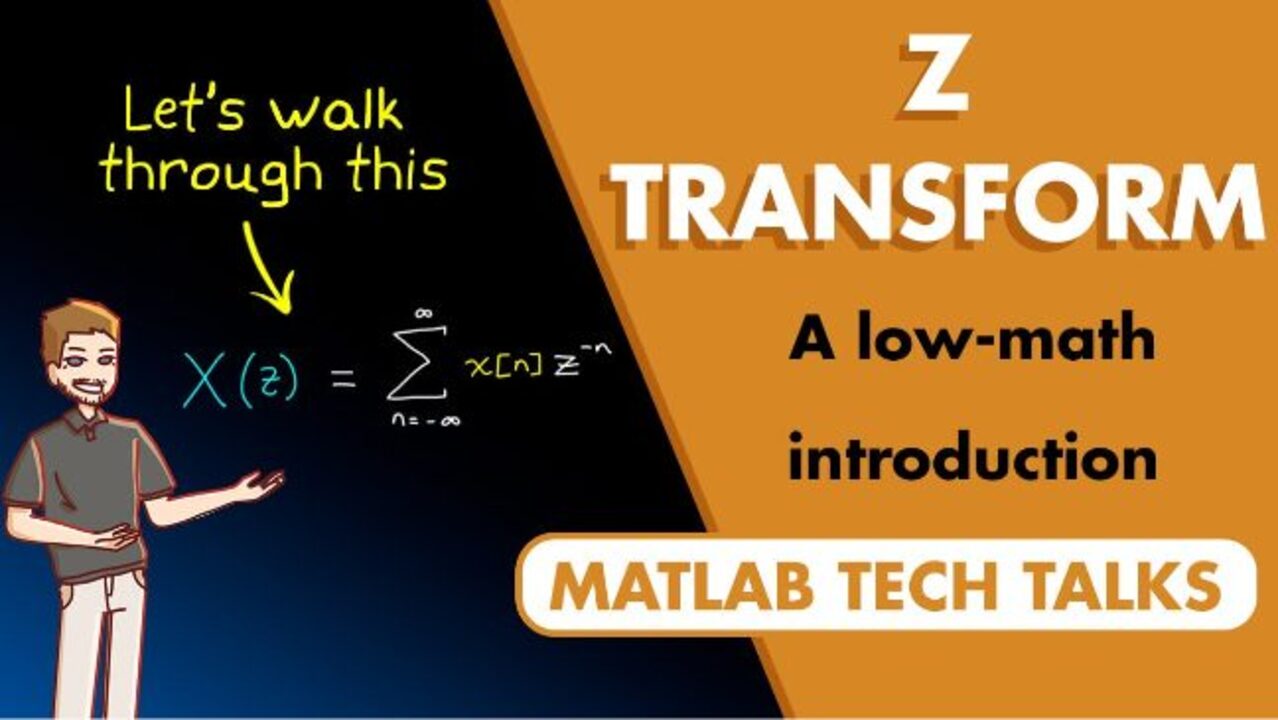
The Z-transform, or "Zed transform," depending on your pronunciation, is a mathematical tool that converts discrete time-domain signals or systems into its Z-domain representation. And this is what the two-sided Z-transform equation looks like. And we can interpret it like this.

We start with a time-domain signal that is sampled periodically where n is the sample number. We then multiply each sample by this variable, z, raised to the negative sample number. And then we sum the result across the entire signal. The output, x, is now a function of this new variable, z.

So mathematically, this equation is pretty straightforward. It's just a bunch of multiplications and additions. And I'm going to show you how to solve this equation for a few different signals in this video. However, understanding how to solve the math of the Z-transform isn't really the important part. The important part, I think, is understanding why the math is the way that it is and what are we actually doing when we take the Z-transform of a signal. And so that's what we're going to spend most of the time on in this video. So I hope you stick around for it.

I'm Brian. And welcome to a MATLAB Tech Talk. To begin, let's look at how we can solve the Z-transform for different discrete time signals and systems. So let's start with a system. And let's say that we apply a discrete time impulse to it. That means that the input has a value of 1 for the first time step and then 0 for all subsequent time steps. The system is affected by that input in some way and then outputs a signal, which we measure with a digital sensor. So it's a discrete time output as well.

For the first system that we want to look at, let's just say that it's a straight pass-through. So it's a value of 1 in the time domain. This means that the output is the exact same as the input. So the question is, what is the Z-domain representation of this system? And to find that, we apply the Z-transform to the output data.

Now, there is no data for negative n-values since the system that produced the data is causal and, therefore, only marches forward in time. Therefore, we can start the summation at n equals 0. And for n equals 0, the time-domain signal has a value of 1. And we multiply that by z to the negative 0, which is also 1.

And now we add to that the time-domain signal at n equals 1 times z to the minus 1, which results in a 0. And then we continue to add additional terms until n equals infinity. However, since the time-domain signal is 0 everywhere else, the final result is just 1. So the Z-domain representation of this system is also 1.

But now let's say that the system actually delays the input by one sample. It's a one-sample delay. In this case, the impulse response is also delayed by one sample. And the Z-transform is 0 times z to the minus 0 plus 1 times z to the minus 1 plus 0 times z to the minus 2, and so on. So a unit delay in the Z-domain is just z to the negative 1. And if the delay was two samples, then the Z-transform would produce z to the minus 2. In this way, a delay of n samples would just be z to the minus n.

So now let's assume that the system is actually an integrator. This means that the output is just the integral of the input, which produces a value of 1 for all time. Here, if we multiply each sample by its corresponding z variable and then sum them all up, we see that the result is this infinite geometric series, z to the minus 0 plus z to the minus 1 plus z to the minus 2, and so on.

Now, working with an infinite series like this isn't terribly convenient. And so we can use a little algebra and refactor this into this ratio of polynomials. So this is the Z-domain representation of an integrator.

Now, finally, we can also take the Z-transform directly on a difference equation. For example, let's say that the system can be described by this difference equation, where the input is just some arbitrary signal u and the output is y. We can take the Z-transform of both sides of this equation.

Now, to find the Z-transform of y of n, we just plug it into the equation. But since that's literally the definition of the Z-transform, the output is just y of z. Same goes for u of n. It becomes u of z.

Now, for the middle term, we're adding 0.5 times the output, y. But that output is delayed by one sample. And we know that a delay is just z inverse. So this becomes 0.5 times a delayed y of z. And now we can put them all together. And with a little algebra, we can get the Z-domain representation of this difference equation.

So hopefully, you can see that solving the Z-transform is pretty straightforward whether you have discrete time data or a different equation. But again, the question that I want to answer isn't really how to solve this math. It's, what is the math actually doing? What is z? And why are we multiplying the time data by it?

So to understand the essence of the Z-transform, I actually think it's helpful to first talk about the discrete-time Fourier transform. The discrete-time Fourier transform converts discrete signals in the time domain to the frequency domain. That is, it represents a signal in terms of its frequency content.

And you can see that it's pretty similar to the Z-transform. In both cases, we're multiplying the time signal by some other signal and summing the result. So I think that if we can understand what the DTFT is doing, we can better understand what the Z-transform is doing.

And to show you what I mean, let's walk through the discrete-time Fourier transform with this MATLAB app that I created. This is a discrete-time signal, x of n. And we can tell just by looking at the data that the signal is probably made up of a single frequency-- at least, one dominating frequency.

So we might ask ourselves, how can we determine what this frequency is if this sampled data is all we have access to? And one way to do this is to compare the data with another signal of a known frequency and see if the two are correlated. If we find the right frequency, then we should reasonably expect the two signals to be highly correlated, whereas other frequencies will be less correlated. And mathematically, here's how we can approach this.

To get a sense of correlation, we can multiply the data signal by the probing signal and then sum the result. When the frequencies are off from each other, like they are here, there's going to be times when both signals are positive or both are negative. And when you multiply these, the result is positive and they add to the total sum.

But when the two signals are of opposite sign, the product is negative and it subtracts from the total. And these adding and subtracting values will tend to cancel out over many samples. And the result, therefore, stays low. So there's less correlation.

We can see here that the sum across these 20 samples at a frequency of 0.2 radians per sample is just about 0. But watch what happens as the signals get closer in frequency. A larger portion of the two signals will start to match signs, which produces more adding values. And then the summation is going to get larger. And we can see here that at 0.41 radians per sample, the summation is about 5.

And then if we keep continuing, we get to the point where they line up perfectly and the two signals are perfectly correlated and the sum is the highest it can be, about 10 for 0.5 radians per sample. And then as we pass through that matching frequency, the result gets low again. So in this way, we're sweeping across all of the possible frequencies. And we're getting a graph that shows how closely our data signal correlates to all of these different probing frequencies.

Now, the signal that we're analyzing is a pure frequency signal. But as you can see, we're claiming there is correlation to these other frequencies as well. And this is the result of the finite length of data. There wasn't enough data to ensure perfect cancellation of the positive and negative signals, especially when the frequencies are close.

But watch as I increase the number of data points. We're giving this whole process more chances to cancel terms. And therefore, the peak at the true frequency gets sharper and taller. It's already off my chart. And if I had infinite data, the results would be a perfectly sharp infinite peak at this one frequency. So in this way, more data means more accurate understanding of the frequency makeup of a periodic signal since there is less leakage across the frequency bands.

So we got there. We found the frequency by multiplying the signal by a cosine wave and summing the results. However, a cosine wave on its own isn't good enough because it has a fixed phase. And the frequencies in the original signal can occur at different phases. If the phase of the data signal is different than the phase of the probing signal, then there's going to be lower correlation between the two. And we can see that as I add phase to the frequency in the original signal. The correlation with the cosine wave starts to drop, as there are now some positive and some negative terms in the product.

And at one point, the correlation disappears completely at the real frequency. And clearly, this isn't good because, as we can see, the frequency is still there in the data. Therefore, instead of probing with a single wave, we can probe the signal with two waves that are offset from each other, a cosine and a sine wave. And to separate them from each other, we can make the sine wave an imaginary signal.

Now, as we adjust the phase of the original signal, we get two responses, a real component-- that is, the correlation to a cosine wave-- and an imaginary component-- that is, the correlation to a sine wave. Now as I adjust the phase of the original signal, we can see that the correlation is trading off between the real and imaginary components. The magnitude of the total correlation is the absolute value of this complex signal. And the phase shift is the argument of the complex signal.

So we're actually multiplying the discrete-time signal by cosine omega n plus i sine omega n. But we can simplify this equation by recognizing that cosine omega n plus i sine omega n is just equal to e to the i omega n. And the convention is to make the exponent negative, which doesn't change the overall idea of the equation. It just swaps negative and positive frequencies.

And check this out. We've arrived at the discrete-time Fourier transform. And that's pretty cool. Hopefully, you can see how this equation is calculating how correlated the time-domain signal is with all of the different frequencies by just multiplying it with sines and cosines and then summing the result.

Analyzing signals like this is useful. However, sometimes we want to know more than just the frequency content of a signal. We also want to understand something about the system itself that generated that signal. If we could understand the system, then not only do we understand the output given some input, but we can predict what the output would be for different inputs. And we could figure out how to manipulate the system in order to get the output that we desire. And an understanding of the system itself is where the Z-transform comes in.

Mathematically, the Z-transform is exactly the same as the discrete-time Fourier transform except in addition to the e to the minus i omega n term, we also multiply it by an r to the minus n term. r is a positive real number. And when you raise r to the exponent negative n, you get an exponential curve. And when r is less than 1, the curve increases exponentially. And when r is greater than 1, the curve decreases exponentially.

So we can think of the Z-transform as a function that is looking for the correlation between the discrete-time signal and both sinusoids from the e term and exponentials from the r term. And if we combine these two probing signals together and simplify it a bit by pulling out the negative n exponent, we get r times e to the i omega, and all of that raised to the minus n. And now we can just claim that a new variable that we call z equals r times e to the i omega. And we've reached the definition of the Z-transform.

Now, why is this important for understanding the system itself? Well, if a system can be modeled as a linear, shift-invariant difference equation, then we can guarantee something about the response-- namely, that the output will contain both frequency content and exponential content because the solution to a linear, shift-invariant difference equation contains both of those components. And if we understand the frequency and exponential makeup of the response given a known input, then we can know exactly the system that generated that response.

Imagine if the impulse response of a system looked like this pure exponential decay. It doesn't really make sense to transform this with a discrete-time Fourier transform. We are going to get frequency content. But it doesn't really mean much because it's not actually representing the dynamics that created this signal. Ideally, we would want to know that there are no oscillations in this signal. There's no important frequency content. But instead, it's just a pure exponential decay because we know what kind of a linear system produces an impulse response that is a pure exponential decay.

So if we're looking for exponentials in the signal, it might make sense to approach this problem just like we did with the discrete-time Fourier transform. That is, let's probe this signal with different exponential functions and see if we can determine which exponentials exist within the signal. And mathematically, this is what the Z-transform is doing. We're probing the data signal with both e to the minus i omega n and r to the negative n to see how well correlated it is to different combinations of oscillations and exponentials. But this simple additional term, r to the minus n, adds some new problems that we didn't encounter with the discrete-time Fourier transform-- namely, convergence.

For example, let's take the exponentially decreasing impulse response. And let's set omega equals 0 in the Z-transform. And so we're really just multiplying by r to the minus n and then summing the result. When r is greater than 1, then our probing signal also decays exponentially. And if we multiply these two signals together, we get an even stronger decay. And the sum is just some finite value. It's not very important what this number is.

But as we start to decrease r, the probing signal starts to decay less quickly. The product of the two is also decaying less quickly. And so the summation is growing. It's still just a boring finite number, though. But at some point, the probing signal grows at the exact same rate that the time signal decays. And when that happens, the product is just a perfectly flat line. And the summation right at this point becomes infinite. It no longer converges.

It is this infinite value that tells us that we have perfectly matched the exponential. There is a pole here since the summation reaches infinity. And in this case, the pole is at a value r less than 1, which means that this is a stable system. The energy in x of n exponentially decays over time.

So the Z-transform is really just sweeping through a bunch of different frequencies and exponentials to see where the summation reaches infinity, called poles. And it's also looking for where the summation is 0, called zeros. But we're going to talk more about poles and zeros in the Z-domain video.

So this is all good except that there's a small problem that can cause confusion. If we keep decreasing r, then the probing signal grows faster than the time signal decays. And the summation is, well, still infinity. In fact, it's even more infinite, which I know doesn't make any sense. But it's growing faster.

So we can't really make the claim that the interesting result only occurs when the summation doesn't converge to a finite value. It's only right at the moment that we go from convergence to nonconvergence that gives us insight into which exponentials exist in the signal. So this region of convergence is important because outside of the region, the results don't make any sense. And this actually becomes an issue if we want to take the Z-transform of finite discrete data. If we only have finite data, then the summation will always converge except for maybe at z equals 0 and z equals infinity.

Even in this example, if our data only has these 20 samples, then you can imagine that this summation of this blue line here is very much not infinity. So we can't tell if we've matched the exponential content of a finite signal by looking at when the result goes to infinity-- that is, unless we make an assumption about what the data is doing for the rest of time.

Remember, at the beginning, we did take the Z-transform on finite data. But in each case, I made an assumption about the future data-- namely, that it was 0, or it was constant. Without that infinite data, the Z-transform just isn't as useful as the Fourier transform.

In fact, this is why in MATLAB, the fast Fourier transform function can operate on finite data. But there isn't a corresponding Z-transform function that will do the same. The Z-trans function requires a system model in order to have an understanding of that infinite data.

But despite that limitation, the Z-transform is still really powerful compared to the discrete-time Fourier transform. With the Z-transform, we're analyzing the system that created the data by looking at frequency and exponential content. With the Fourier transform, were analyzing the signal that the system produced. And we do so just by looking at frequency content.

I hope all of this information has helped you understand the Z-transform. We're going to be making a video on the Z-domain that answers the question, why are we even going into the Z-domain in the first place? What's so special about it? And we'll link to that here when it's published.

But in the meantime, you can find all of the Tech Talk videos across many different topics nicely organized at MathWorks.com. And if you liked this video, then you might be interested to learn how a discrete-time delay can be represented in the S-domain using a Padé approximation. So I hope you check that out.

Thanks for watching. And I'll see you next time.