Analysis of Biquad Yagi for Wi-Fi Applications

This example shows how to analyze the performance of a customized Yagi-Uda antenna. Biquad Yagi antenna is popularly used in Wi-Fi applications.

Define Parameters

Design the biquad yagi antenna to operate at 2.4 GHz. Use dimensions of 28.9 mm element for the first parasitic element followed by three other elements of same dimension, then 35 mm driven element and a 44.6 mm reflector at the rear. Define the design parameters of the antenna as provided.

ref = biquad(Tilt=90,ArmLength=44.6e-3,Width=1.6e-3);      % Reflector
exct = biquad(Tilt=90,ArmLength=35e-3,Width=1.6e-3);     % Driven element
direct1 = biquad(Tilt=90,ArmLength=28.9e-3,Width=0.9e-3);  % Director1
direct2 = biquad(Tilt=90,ArmLength=28.9e-3,Width=0.9e-3);  % Director2
direct3 = biquad(Tilt=90,ArmLength=28.9e-3,Width=0.9e-3);  % Director3
direct4 = biquad(Tilt=90,ArmLength=28.9e-3,Width=0.9e-3);  % Director4

Create Biquad Yagi Antenna

Space the parasitic elements 24 mm from driven element and the reflector 35 mm from the driven element. You can increase and decrease the length of the Boom and, you can move the Boom by changing the BoomOffset property. Create a quadCustom antenna using the parameters defined.

ant =  quadCustom(Exciter=exct,Director={direct1,direct2,direct3,direct4},...
    DirectorSpacing=24e-3,Reflector={ref},ReflectorSpacing=35e-3,...
    BoomOffset=[0 0.04 0.060],BoomLength=0.2,BoomWidth=0.002);
figure
ant.Tilt = 180;
ant.TiltAxis = [0 1 1];
show(ant)
title("Biquad Yagi Antenna");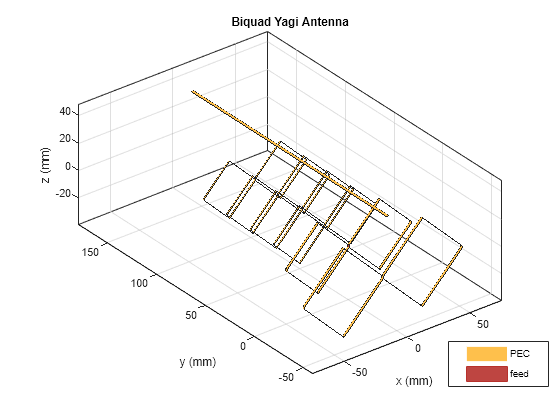

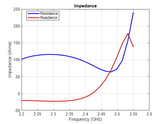
Calculate Antenna Impedance

Calculate the antenna impedance over the frequency range of 2.2 GHz to 2.55 GHz. From the figure, observe the antenna resonates around 2.4 GHz.

figure
impedance(ant,linspace(2.2e9,2.55e9,21));

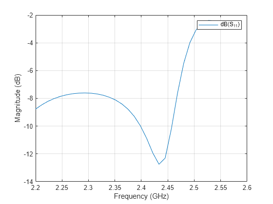
Plot Reflection Coefficient

Plot the reflection coefficient for this antenna over the band and a reference impedance of 50 ohms.

figure
s = sparameters(ant,linspace(2.2e9,2.55e9,31));
rfplot(s);

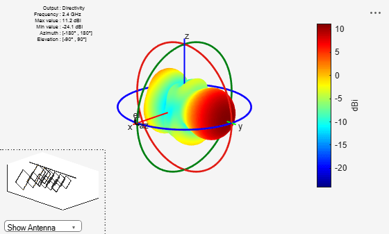
Calculate and Plot Pattern

Plot the radiation pattern for this antenna at the frequency of best match in the band.

figure
pattern(ant,2.4e9);

Current Distribution

Plot the surface current distribution for this antenna at 2.4 GHz.

figure
current(ant,2.4e9,Scale="log10");