coeffs
Get filter coefficients
Syntax
Description
Examples
Create a graphicEQ and then call coeffs to get its coefficients. The coefficients are returned as second-order sections. The dimensions of B are 3-by-(M * EQOrder / 2), where M is the number of bandpass equalizers. The dimensions of A are 2-by-(M * EQOrder / 2).
fs = 44.1e3;
x = 0.1*randn(fs*5,1);
equalizer = graphicEQ('SampleRate',fs, ...
                      'Gains',[-10,-10,10,10,-10,-10,10,10,-10,-10], ...
                      'EQOrder',2);

[B,A] = coeffs(equalizer);
Compare the output of the filter function using coefficients B and A with the output of graphicEQ.
y = x;
for section = 1:equalizer.EQOrder/2
     for i = 1:numel(equalizer.Gains)
        y = filter(B(:,i*section),A(:,i*section),y);
     end
end
audioOut_filter = y;

audioOut = equalizer(x);

subplot(2,1,1)
plot(abs(fft(audioOut)))
title('graphicEQ')
ylabel('Magnitude Response')

subplot(2,1,2)
plot(abs(fft(audioOut_filter)))
title('Filter function')
xlabel('Bin')
ylabel('Magnitude Response')

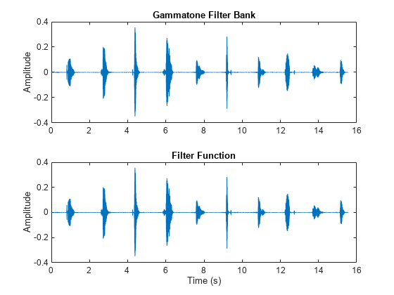
Create the default gammatoneFilterBank, and then call coeffs to get its coefficients. Each gammatone filter is an eighth-order IIR filter composed of a cascade of four second-order sections. The size of B is 4-by-3-by-NumFilters. The size of A is 4-by-2-by-NumFilters.
[audioIn,fs] = audioread('Counting-16-44p1-mono-15secs.wav');

gammaFiltBank = gammatoneFilterBank('SampleRate',fs);

[B,A] = coeffs(gammaFiltBank);
Compare the output of the filter function using coefficients B and A with the output of gammaFiltBank. For simplicity, compare output from channel eight only.
channelToCompare = 8;
y1 = filter(B(1,:,channelToCompare),[1,A(1,:,channelToCompare)],audioIn);
y2 = filter(B(2,:,channelToCompare),[1,A(2,:,channelToCompare)],y1);
y3 = filter(B(3,:,channelToCompare),[1,A(3,:,channelToCompare)],y2);
audioOut_filter = filter(B(4,:,channelToCompare),[1,A(4,:,channelToCompare)],y3);

audioOut = gammaFiltBank(audioIn);

t = (0:(size(audioOut,1)-1))'/fs;

subplot(2,1,1)
plot(t,audioOut(:,channelToCompare))
title('Gammatone Filter Bank')
ylabel('Amplitude')

subplot(2,1,2)
plot(t,audioOut_filter)
title('Filter Function')
xlabel('Time (s)')
ylabel('Amplitude')
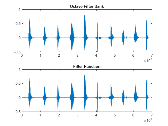
Create the default octaveFilterBank, and then call coeffs to get its coefficients. The coefficients are returned as second-order sections. The dimensions of B and A are T-by-3-by-M, where T is the number of sections and M is the number of filters.
[audioIn,fs] = audioread('Counting-16-44p1-mono-15secs.wav');

octFiltBank = octaveFilterBank('SampleRate',fs);

[B,A] = coeffs(octFiltBank);
Compare the output of the filter function using coefficients B and A with the output of octaveFilterBank. For simplicity, compare output from channel five only.
channelToCompare = 5;

audioOut_filter = filter(B(1,:,channelToCompare),A(1,:,channelToCompare),audioIn);
audioOut = octFiltBank(audioIn);

subplot(2,1,1)
plot(audioOut(:,channelToCompare))
title('Octave Filter Bank')

subplot(2,1,2)
plot(audioOut_filter)
title('Filter Function')