Analyzing Illumina Bead Summary Gene Expression Data
This example shows how to analyze Illumina® BeadChip gene expression summary data using MATLAB® and Bioinformatics Toolbox™ functions.
Introduction
This example shows how to import and analyze gene expression data from the Illumina BeadChip microarray platform. The data set in the example is from the study of gene expression profiles of human spermatogenesis by Platts et al. [1]. The expression levels were measured on Illumina Sentrix Human 6 (WG6) BeadChips.
The data from most microarray gene expression experiments generally consists of four components: experiment data values, sample information, feature annotations, and information about the experiment. This example uses microarray data, constructs each of the four components, assembles them into an ExpressionSet object, and finds the differentially expressed genes. For more examples about the ExpressionSet class, see Working with Objects for Microarray Experiment Data.
Importing Experimental Data from the GEO Database
Samples were hybridized on three Illumina Sentrix Human 6 (WG6) BeadChips. Retrieve the GEO Series data GSE6967 using getgeodata function.
TNGEOData = getgeodata('GSE6967')
TNGEOData =

  struct with fields:

    Header: [1×1 struct]
      Data: [47293×13 bioma.data.DataMatrix]
The TNGEOData structure contains Header and Data fields. The Header field has two fields, Series and Samples, containing a description of the experiment and samples respectively. The Data field contains a DataMatrix of normalized summary expression levels from the experiment.
Determine the number of samples in the experiment.
nSamples = numel(TNGEOData.Header.Samples.geo_accession)
nSamples =

    13
Inspect the sample titles from the Header.Samples field.
TNGEOData.Header.Samples.title'
ans =

  13×1 cell array

    {'Teratozoospermic individual: Sample T2'}
    {'Teratozoospermic individual: Sample T1'}
    {'Teratozoospermic individual: Sample T6'}
    {'Teratozoospermic individual: Sample T4'}
    {'Teratozoospermic individual: Sample T8'}
    {'Normospermic individual: Sample N11'   }
    {'Teratozoospermic individual: Sample T3'}
    {'Teratozoospermic individual: Sample T7'}
    {'Teratozoospermic individual: Sample T5'}
    {'Normospermic individual: Sample N6'    }
    {'Normospermic individual: Sample N12'   }
    {'Normospermic individual: Sample N5'    }
    {'Normospermic individual: Sample N1'    }
For simplicity, extract the sample labels from the sample titles.
sampleLabels = cellfun(@(x) char(regexp(x, '\w\d+', 'match')),...
                TNGEOData.Header.Samples.title, 'UniformOutput',false)
sampleLabels =

  1×13 cell array

  Columns 1 through 7

    {'T2'}    {'T1'}    {'T6'}    {'T4'}    {'T8'}    {'N11'}    {'T3'}

  Columns 8 through 13

    {'T7'}    {'T5'}    {'N6'}    {'N12'}    {'N5'}    {'N1'}
Importing Expression Data from Illumina BeadStudio Summary Files
Download the supplementary file GSE6967_RAW.tar and unzip the file to access the 13 text files produced by the BeadStudio software, which contain the raw, non-normalized bead summary values.
The raw data files are named with their GSM accession numbers. For this example, construct the file names of the text data files using the path where the text files are located.
rawDataFiles = cell(1,nSamples);
for i = 1:nSamples
    rawDataFiles {i} = [TNGEOData.Header.Samples.geo_accession{i} '.txt'];
end
Set the variable rawDataPath to the path and directory to which you extracted the data files.
rawDataPath = 'C:\Examples\illuminagedemo\GSE6967';
Use the ilmnbsread function to read the first of the summary files and store the content in a structure.
rawData = ilmnbsread(fullfile(rawDataPath, rawDataFiles{1}))
rawData =

  struct with fields:

             Header: [1×1 struct]
           TargetID: {47293×1 cell}
        ColumnNames: {1×8 cell}
               Data: [47293×8 double]
    TextColumnNames: {}
           TextData: {}
Inspect the column names in the rawData structure.
rawData.ColumnNames'
ans =

  8×1 cell array

    {'MIN_Signal-1412091085_A' }
    {'AVG_Signal-1412091085_A' }
    {'MAX_Signal-1412091085_A' }
    {'NARRAYS-1412091085_A'    }
    {'ARRAY_STDEV-1412091085_A'}
    {'BEAD_STDEV-1412091085_A' }
    {'Avg_NBEADS-1412091085_A' }
    {'Detection-1412091085_A'  }
Determine the number of target probes.
nTargets = size(rawData.Data, 1)
nTargets =

       47293
Read the non-normalized expression values (Avg_Signal), the detection confidence limits and the Sentrix chip IDs from the summary data files. The gene expression values are identified with Illumina probe target IDs. You can specify the columns to read from the data file.
rawMatrix = bioma.data.DataMatrix(zeros(nTargets, nSamples),...
                                  rawData.TargetID, sampleLabels);
detectionConf = bioma.data.DataMatrix(zeros(nTargets, nSamples),...
                                      rawData.TargetID, sampleLabels);
chipIDs = categorical([]);

for i = 1:nSamples
    rawData =ilmnbsread(fullfile(rawDataPath, rawDataFiles{i}),...
                                'COLUMNS', {'AVG_Signal', 'Detection'});
    chipIDs(i) = regexp(rawData.ColumnNames(1), '\d*', 'match', 'once');
    rawMatrix(:, i) = rawData.Data(:, 1);
    detectionConf(:,i) = rawData.Data(:,2);
end
There are three Sentrix BeadChips used in the experiment. Inspect the Illumina Sentrix BeadChip IDs in chipIDs to determine the number of samples hybridized on each chip.
summary(chipIDs)

samplesChip1 = sampleLabels(chipIDs=='1412091085')
samplesChip2 = sampleLabels(chipIDs=='1412091086')
samplesChip3 = sampleLabels(chipIDs=='1477791158')
<strong>chipIDs</strong>: 1×13 categorical

     <strong>1412091085</strong>      <strong>1412091086</strong>      <strong>1477791158</strong>      <strong><undefined></strong>
     6               4               3               0

samplesChip1 =

  1×6 cell array

    {'T2'}    {'T1'}    {'T6'}    {'T4'}    {'T8'}    {'N11'}


samplesChip2 =

  1×4 cell array

    {'T3'}    {'T7'}    {'T5'}    {'N6'}


samplesChip3 =

  1×3 cell array

    {'N12'}    {'N5'}    {'N1'}
Six samples (T2, T1, T6, T4, T8, and N11) were hybridized to six arrays on the first chip, four samples (T3, T7, T5, and N6) on the second chip, and three samples (N12, N5, and N1) on the third chip.
Normalizing the Expression Data
Use a boxplot to view the raw expression levels of each sample in the experiment.
logRawExprs = log2(rawMatrix);

maboxplot(logRawExprs, 'Orientation', 'horizontal')
ylabel('Sample Labels')
xlabel('log2(Expression Value)')
title('Before Normalization')
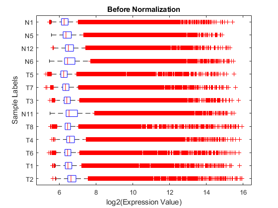
The difference in intensities between samples on the same chip and samples on different chips does not seem too large. The first BeadChip, containing samples T2, T1, T6, T4, T8 and N11, seems to be slightly more variable than others.
Using MA and XY plots to do a pairwise comparison of the arrays on a BeadChip can be informative. On an MA plot, the average (A) of the expression levels of two arrays are plotted on the x axis, and the difference (M) in the measurement on the y axis. An XY plot is a scatter plot of one array against another. This example uses the helper function maxyplot to plot MAXY plots for a pairwise comparison of the three arrays on the first chip hybridized with teratozoospermic samples (T2, T1 and T6).
Note: You can also use the mairplot function to create the MA or IR (Intensity/Ratio) plots for comparison of specific arrays.
inspectIdx = 1:3;
maxyplot(rawMatrix, inspectIdx)
sgtitle('Before Normalization')
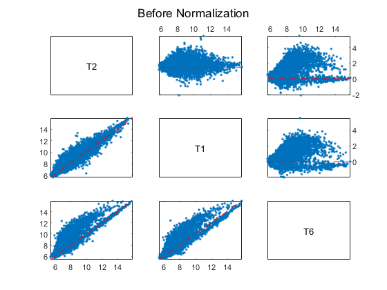
In an MAXY plot, the MA plots for all pairwise comparisons are in the upper-right corner. In the lower-left corner are the XY plots of the comparisons. The MAXY plot shows the two arrays, T1 and T2, to be quite similar, while different from the other array, T6.
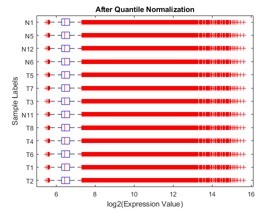
The expression box plots and MAXY plots reveal that there are differences in expression levels within chips and between chips; hence, the data requires normalization. Use the quantilenorm function to apply quantile normalization to the raw data.
Note: You can also try invariant set normalization using the mainvarsetnorm function.
normExprs = rawMatrix;
normExprs(:, :) = quantilenorm(rawMatrix.(':')(':'));

log2NormExprs = log2(normExprs);
Display and inspect the normalized expression levels in a box plot.
figure;
maboxplot(log2NormExprs, 'ORIENTATION', 'horizontal')
ylabel('Sample Labels')
xlabel('log2(Expression Value)')
title('After Quantile Normalization')
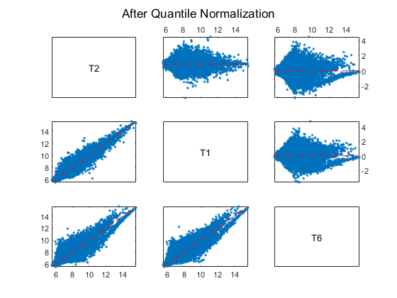
Display and inspect the MAXY plot of the three arrays (T2, T1 and T6) on the first chip after the normalization.
maxyplot(normExprs, inspectIdx)
sgtitle('After Quantile Normalization')
Many of the genes in this study are not expressed, or have only small variability across the samples.
First, you can remove genes with very low absolute expression values by using genelowvalfilter.
[mask, log2NormExprs] = genelowvalfilter(log2NormExprs);
detectionConf = detectionConf(mask, :);
Second, filter out genes with a small variance across samples using genevarfilter.
[mask, log2NormExprs] = genevarfilter(log2NormExprs);
detectionConf = detectionConf(mask, :);
Importing Feature Metadata from a BeadChip Annotation File
Microarray manufacturers usually provide annotations of a collection of features for each type of chip. The chip annotation files contain metadata such as the gene name, symbol, NCBI accession number, chromosome location and pathway information. Before assembling an ExpressionSet object for the experiment, obtain the annotations about the features or probes on the BeadChip. You can download the Human_WG-6.csv annotation file for Sentrix Human 6 (WG6) BeadChips from the Support page at the Illumina web site and save the file locally. Read the annotation file into MATLAB as a dataset array. Set the variable annotPath to the path and directory to which you downloaded the annotation file.
annotPath = fullfile('C:\Examples\illuminagedemo\Annotation');
WG6Annot = dataset('xlsfile', fullfile(annotPath, 'Human_WG-6.csv'));
Inspect the properties of this dataset array.
get(WG6Annot)
       Description: ''
    VarDescription: {}
             Units: {}
          DimNames: {'Observations'  'Variables'}
          UserData: []
          ObsNames: {}
          VarNames: {1×13 cell}
Get the names of variables describing the features on the chip.
fDataVariables = get(WG6Annot, 'VarNames')
fDataVariables =

  1×13 cell array

  Columns 1 through 5

    {'Search_key'}    {'Target'}    {'ProbeId'}    {'Gid'}    {'Transcript'}

  Columns 6 through 10

    {'Accession'}    {'Symbol'}    {'Type'}    {'Start'}    {'Probe_Sequence'}

  Columns 11 through 13

    {'Definition'}    {'Ontology'}    {'Synonym'}
Check the number of probe target IDs in the annotation file.
numel(WG6Annot.Target)
ans =

       47296
Because the expression data in this example is only a small set of the full expression values, you will work with only the features in the DataMatrix object log2NormExprs. Find the matching features in log2NormExprs and WG6Annot.Target.
[commTargets, fI, WGI] = intersect(rownames(log2NormExprs), WG6Annot.Target);
Building an ExpressionSet Object for Experimental Data
You can store the preprocessed expression values and detection limits of the annotated probe targets as an ExptData object.
fNames = rownames(log2NormExprs);
TNExptData = bioma.data.ExptData({log2NormExprs(fI, :), 'ExprsValues'},...
                                 {detectionConf(fI, :), 'DetectionConfidences'})
TNExptData =

Experiment Data:
  42313 features,  13 samples
  2 elements
  Element names: ExprsValues, DetectionConfidences
Building an ExpressionSet Object for Sample Information
The sample data in the Header.Samples field of the TNGEOData structure can be overwhelming and difficult to navigate through. From the data in Header.Samples field, you can gather the essential information about the samples, such as the sample titles, GEO sample accession numbers, etc., and store the sample data as a MetaData object.
Retrieve the descriptions about sample characteristics.
sampleChars = cellfun(@(x) char(regexp(x, '\w*tile', 'match')),...
               TNGEOData.Header.Samples.characteristics_ch1, 'UniformOutput', false)
sampleChars =

  1×13 cell array

  Columns 1 through 4

    {'Infertile'}    {'Infertile'}    {'Infertile'}    {'Infertile'}

  Columns 5 through 8

    {'Infertile'}    {'Fertile'}    {'Infertile'}    {'Infertile'}

  Columns 9 through 13

    {'Infertile'}    {'Fertile'}    {'Fertile'}    {'Fertile'}    {'Fertile'}
Create a dataset array to store the sample data you just extracted.
sampleDS = dataset({TNGEOData.Header.Samples.geo_accession', 'GSM'},...
                   {strtok(TNGEOData.Header.Samples.title)', 'Type'},...
                   {sampleChars', 'Characteristics'}, 'obsnames', sampleLabels')
sampleDS =

           GSM                  Type                        Characteristics
    T2     {'GSM160620'}        {'Teratozoospermic'}        {'Infertile'}
    T1     {'GSM160621'}        {'Teratozoospermic'}        {'Infertile'}
    T6     {'GSM160622'}        {'Teratozoospermic'}        {'Infertile'}
    T4     {'GSM160623'}        {'Teratozoospermic'}        {'Infertile'}
    T8     {'GSM160624'}        {'Teratozoospermic'}        {'Infertile'}
    N11    {'GSM160625'}        {'Normospermic'    }        {'Fertile'  }
    T3     {'GSM160626'}        {'Teratozoospermic'}        {'Infertile'}
    T7     {'GSM160627'}        {'Teratozoospermic'}        {'Infertile'}
    T5     {'GSM160628'}        {'Teratozoospermic'}        {'Infertile'}
    N6     {'GSM160629'}        {'Normospermic'    }        {'Fertile'  }
    N12    {'GSM160630'}        {'Normospermic'    }        {'Fertile'  }
    N5     {'GSM160631'}        {'Normospermic'    }        {'Fertile'  }
    N1     {'GSM160632'}        {'Normospermic'    }        {'Fertile'  }
Store the sample metadata as an object of the MetaData class, including a short description for each variable.
TNSData = bioma.data.MetaData(sampleDS,...
    {'Sample GEO accession number',...
    'Spermic type',...
    'Fertility characteristics'})
TNSData =

Sample Names:
    T2, T1, ...,N1 (13 total)
Variable Names and Meta Information:
                       VariableDescription
    GSM                {'Sample GEO accession number'}
    Type               {'Spermic type'               }
    Characteristics    {'Fertility characteristics'  }
Building an ExpressionSet Object for Feature Annotations
The collection of feature metadata for Sentrix Human 6 BeadChips is large and diverse. Select information about features that are unique to the experiment and save the information as a MetaData object. Extract annotations of interest, for example, Accession and Symbol.
fIdx = ismember(fDataVariables, {'Accession', 'Symbol'});

featureAnnot = WG6Annot(WGI, fDataVariables(fIdx));
featureAnnot = set(featureAnnot, 'ObsNames', WG6Annot.Target(WGI));
Create a MetaData object for the feature annotation information with brief descriptions about the two variables of the metadata.
WG6FData = bioma.data.MetaData(featureAnnot, ...
            {'Accession number of probe target', 'Gene Symbol of probe target'})
WG6FData =

Sample Names:
    GI_10047089-S, GI_10047091-S, ...,hmm9988-S (42313 total)
Variable Names and Meta Information:
                 VariableDescription
    Accession    {'Accession number of probe target'}
    Symbol       {'Gene Symbol of probe target'     }
Building an ExpressionSet Object for Experiment Information
Most of the experiment descriptions in the Header.Series field of the TNGEOData structure can be reorganized and stored as a MIAME object, which you will use to assemble the ExpressionSet object for the experiment.
TNExptInfo = bioma.data.MIAME(TNGEOData)
TNExptInfo =

Experiment Description:
  Author name: Adrian,E,Platts
David,J,Dix
Hector,E,Chemes
Kary,E,Thompson
Robert,,Goodrich
John,C,Rockett
Vanesa,Y,Rawe
Silvina,,Quintana
Michael,P,Diamond
Lillian,F,Strader
Stephen,A,Krawetz
  Laboratory: Wayne State University
  Contact information: Stephen,A,Krawetz
  URL: http://compbio.med.wayne.edu
  PubMedIDs: 17327269
  Abstract: A 82 word abstract is available. Use the Abstract property.
  Experiment Design: A 61 word summary is available. Use the ExptDesign property.
  Other notes:
    {'ftp://ftp.ncbi.nlm.nih.gov/geo/series/GSE6nnn/GSE6967/suppl/GSE6967_RAW.tar'}
Assembling an ExpressionSet Object
Now that you've created all the components, you can create an object of the ExpressionSet class to store the expression values, sample information, chip feature annotations and description information about this experiment.
TNExprSet = bioma.ExpressionSet(TNExptData, 'sData', TNSData,...
                                            'fData', WG6FData,...
                                            'eInfo', TNExptInfo)
TNExprSet =

ExpressionSet
Experiment Data: 42313 features, 13 samples
  Element names: Expressions, DetectionConfidences
Sample Data:
    Sample names:     T2, T1, ...,N1 (13 total)
    Sample variable names and meta information:
        GSM: Sample GEO accession number
        Type: Spermic type
        Characteristics: Fertility characteristics
Feature Data:
    Feature names:     GI_10047089-S, GI_10047091-S, ...,hmm9988-S (42313 total)
    Feature variable names and meta information:
        Accession: Accession number of probe target
        Symbol: Gene Symbol of probe target
Experiment Information: use 'exptInfo(obj)'
Note: The ExprsValues element in the ExptData object, TNExptData, is renamed to Expressions in TNGeneExprSet.
You can save an object of ExpressionSet class as a MAT file for further data analysis.
save TNGeneExprSet TNExprSet
Profiling Gene Expression by Using Permutation T-tests
Load the experiment data saved from the previous section. You will use this data to find differentially expressed genes between the teratozoospermia and normal samples.
load TNGeneExprSet
To identify the differential changes in the levels of transcripts in normospermic Ns and teratozoospermic Tz samples, compare the gene expression values between the two groups of data: Tz and Ns.
TNSamples = sampleNames(TNExprSet);
Tz = strncmp(TNSamples, 'T', 1);
Ns = strncmp(TNSamples, 'N', 1);
nTz = sum(Tz)
nNs = sum(Ns)

TNExprs = expressions(TNExprSet);
TzData = TNExprs(:,Tz);
NsData = TNExprs(:,Ns);
meanTzData = mean(TzData,2);
meanNsData = mean(NsData,2);
groupLabels = [TNSamples(Tz), TNSamples(Ns)];
nTz =

     8


nNs =

     5
Perform a permutation t-test using the mattest function to permute the columns of the gene expression data matrix of TzData and NsData. Note: Depending on the sample size, it may not be feasible to consider all possible permutations. Usually, a random subset of permutations are considered in the case of a large sample size.
Use the nchoosek function in Statistics and Machine Learning Toolbox™ to determine the number of all possible permutations of the samples in this example.
perms = nchoosek(1:nTz+nNs, nTz);
nPerms = size(perms,1)
nPerms =

        1287
Use the PERMUTE option of the mattest function to compute the p-values of all the permutations.
pValues = mattest(TzData, NsData, 'Permute', nPerms);
You can also compute the differential score from the p-values using the following anonymous function [1].
diffscore = @(p, avgTest, avgRef) -10*sign(avgTest - avgRef).*log10(p);
A differential score of 13 corresponds to a p-value of 0.05, a differential score of 20 corresponds to a p-value of 0.01, and a differential score of 30 corresponds to a p-value of 0.001. A positive differential score represents up-regulation, while a negative score represents down-regulation of genes.
diffScores = diffscore(pValues, meanTzData, meanNsData);
Determine the number of genes considered to have a differential score greater than 20. Note: You may get a different number of genes due to the permutation test outcome.
up = sum(diffScores > 20)

down = sum(diffScores < -20)
up =

        3741


down =

        3033
Estimating False Discovery Rate (FDR)
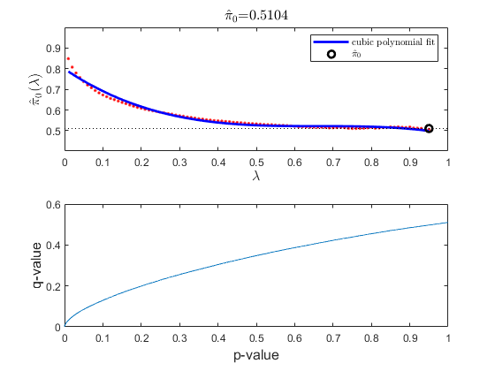
In multiple hypothesis testing, where we simultaneously tests the null hypothesis of thousands of genes, each test has a specific false positive rate, or a false discovery rate (FDR) [2]. Estimate the FDR and q-values for each test using the mafdr function.
figure;
[pFDR, qValues] = mafdr(pValues, 'showplot', true);
diffScoresFDRQ = diffscore(qValues, meanTzData, meanNsData);
Determine the number of genes with an absolute differential score greater than 20. Note: You may get a different number of genes due to the permutation test and the bootstrap outcomes.
sum(abs(diffScoresFDRQ)>=20)
ans =

        3122
Identifying Genes that Are Differentially Expressed
Plot the -log10 of p-values against fold changes in a volcano plot.
diffStruct = mavolcanoplot(TzData, NsData, qValues,...
                                   'pcutoff', 0.01, 'foldchange', 5);
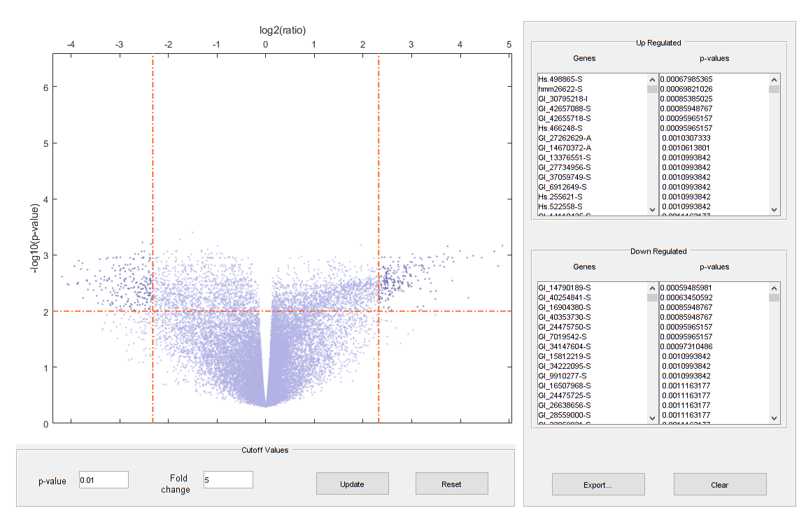
Note: From the volcano plot UI, you can interactively change the p-value cutoff and fold-change limit, and export differentially expressed genes.
Determine the number of differentially expressed genes.
nDiffGenes = numel(diffStruct.GeneLabels)
nDiffGenes =

   451
Get the list of up-regulated genes for the Tz samples compared to the Ns samples.
up_genes = diffStruct.GeneLabels(diffStruct.FoldChanges > 0);
nUpGenes = length(up_genes)
nUpGenes =

   223
Get the list of down-regulated genes for the Tz samples compared to the Ns samples.
down_genes = diffStruct.GeneLabels(diffStruct.FoldChanges < 0);
nDownGenes = length(down_genes)
nDownGenes =

   228
Extract a list of differentially expressed genes.
diff_geneidx = zeros(nDiffGenes, 1);
for i = 1:nDiffGenes
    diff_geneidx(i) = find(strncmpi(TNExprSet.featureNames, ...
                            diffStruct.GeneLabels{i}, length(diffStruct.GeneLabels{i})), 1);
end
You can get the subset of experiment data containing only the differentially expressed genes.
TNDiffExprSet = TNExprSet(diff_geneidx, groupLabels);
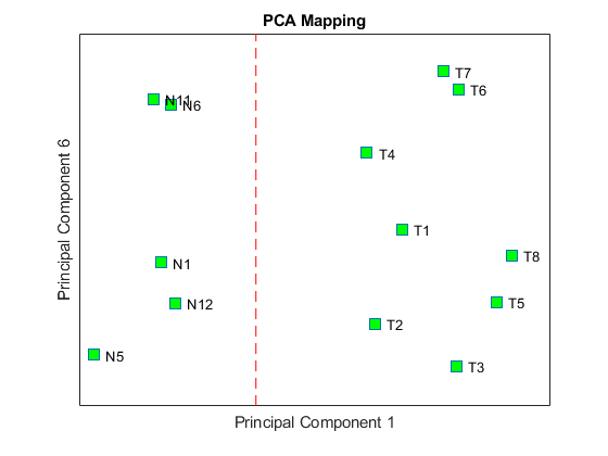
Performing PCA and Clustering Analysis of Significant Gene Profiles
Principal component analysis (PCA) on differentially expressed genes shows linear separability of the Tz samples from the Ns samples.
PCAScore = pca(TNDiffExprSet.expressions);
Display the coefficients of the first and sixth principal components.
figure;
plot(PCAScore(:,1), PCAScore(:,6), 's', 'MarkerSize',10, 'MarkerFaceColor','g');
hold on
text(PCAScore(:,1)+0.02, PCAScore(:,6), TNDiffExprSet.sampleNames)
plot([0,0], [-0.5 0.5], '--r')
ax = gca;
ax.XTick = [];
ax.YTick = [];
ax.YTickLabel = [];
title('PCA Mapping')
xlabel('Principal Component 1')
ylabel('Principal Component 6')
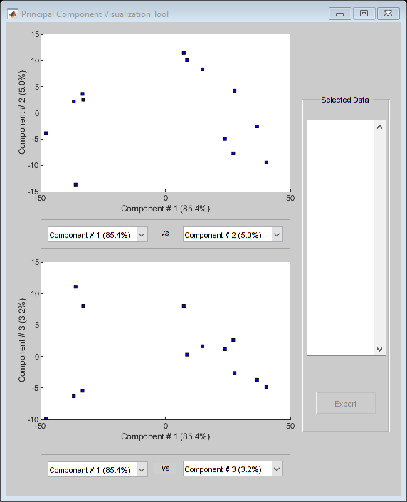
You can also use the interactive tool created by the mapcaplot function to perform principal component analysis.
mapcaplot((TNDiffExprSet.expressions)')
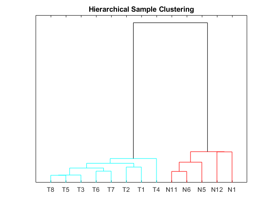
Perform unsupervised hierarchical clustering of the significant gene profiles from the Tz and Ns groups using correlation as the distance metric to cluster the samples.
sampleDist = pdist(TNDiffExprSet.expressions','correlation');
sampleLink = linkage(sampleDist);

figure;
dendrogram(sampleLink, 'labels', TNDiffExprSet.sampleNames,'ColorThreshold',0.5)
ax = gca;
ax.YTick = [];
ax.Box = 'on';
title('Hierarchical Sample Clustering')
Use the clustergram function to create the hierarchical clustering of differentially expressed genes, and apply the colormap redbluecmap to the clustergram.
cmap = redbluecmap(9);
cg = clustergram(TNDiffExprSet.expressions,'Colormap',cmap,'Standardize',2);
addTitle(cg,'Hierarchical Gene Clustering')

Clustering of the most differentially abundant transcripts clearly partitions teratozoospermic (Tz) and normospermic (Ns) spermatozoal RNAs.
References
[1] Platts, A.E., et al., "Success and failure in human spermatogenesis as revealed by teratozoospermic RNAs", Human Molecular Genetics, 16(7):763-73, 2007.
[2] Storey, J.D. and Tibshirani, R., "Statistical significance for genomewide studies", PNAS, 100(16):9440-5, 2003.