chbpnt

Chebyshev-Demko points

Syntax

tau = chbpnt(t,k)
chbpnt(t,k,tol)
[tau,sp] = chbpnt(...)


Description

tau = chbpnt(t,k) are the extreme sites of the Chebyshev spline of order k with knot sequence t. These are particularly good sites at which to interpolate data by splines of order k with knot sequence t because the resulting interpolant is often quite close to the best uniform approximation from that spline space to the function whose values at tau are being interpolated.

chbpnt(t,k,tol) also specifies the tolerance tol to be used in the iterative process that constructs the Chebyshev spline. This process is terminated when the relative difference between the absolutely largest and the absolutely smallest local extremum of the spline is smaller than tol. The default value for tol is .001.

[tau,sp] = chbpnt(...) also returns, in sp, the Chebyshev spline.

Examples

Approximate Square Root Function

Create a knot sequence of ten zeros and ten ones using the augknt function.

k = 10;
t = augknt([0,1],k);

Create a vector of interpolation sites by calculating the Chebyshev-Demko points for the Chebyshev spline of order 10 with knot sequence t.

sites = chbpnt(t,k);

Create a vector of interpolation points by evaluating the function sqrt at the Chebyshev-Demko points. Use the function spapi to interpolate through the evaluated points with a tenth-order spline from the knot sequence t. The knots in t indicate that the spline fit consists of a single polynomial with boundaries at 0 and 1.

interpolationPoints = sqrt(sites);
sp = spapi(t,sites,interpolationPoints)

sp = struct with fields:
      form: 'B-'
     knots: [0 0 0 0 0 0 0 0 0 0 1 1 1 1 1 1 1 1 1 1]
     coefs: [-4.2719e-17 0.8842 -0.7101 2.4484 -1.1869 1.9678 0.3331 0.9940 0.9349 1]
    number: 10
     order: 10
       dim: 1

The structure sp contains the properties of the spline. The coefs field of sp is a vector of coefficients for the polynomial that approximates the square root function in the interval [0,1].

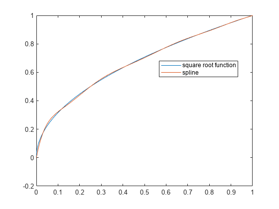
Compare sp and the square root function by displaying them in the same plot.

x = linspace(0,1,1000);

plot(x,sqrt(x))
hold on
fnplt(sp,'-',0.75)
legend(["square root function" "spline"],Location="best")

The plot shows that the spline closely follows the square root function.

Compare Interpolation Points for Runge Function

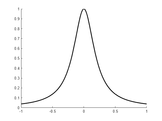
Create an anonymous function for the Runge function and plot it in the interval [-1 1].

runge = @(x) 1./(1+25*x.^2);
figure
hold on
fplot(runge,[-1 1],"k",LineWidth=2);

Use augknt and linspace to create a knot sequence and equally spaced interpolation points in the interval [-1 1]. Evaluate the built-in Runge function runge at the interpolation points.

k = 11;
t = augknt([-1 1],k);
x_es = linspace(-0.99,0.99,k);
y_es = runge(x_es);

Fit a degree-ten polynomial spline with the knot sequence t through the equally spaced interpolation points.

sp_es = spapi(t,x_es,y_es)

sp_es = struct with fields:
      form: 'B-'
     knots: [-1 -1 -1 -1 -1 -1 -1 -1 -1 -1 -1 1 1 1 1 1 1 1 1 1 1 1]
     coefs: [-0.8586 19.5179 -73.4835 169.6651 -275.4870 326.3246 -275.4870 169.6651 -73.4835 19.5179 -0.8586]
    number: 11
     order: 11
       dim: 1

sq_es is a struct that contains the results of the fit. The field coefs contain the coefficients for the degree-ten polynomial.

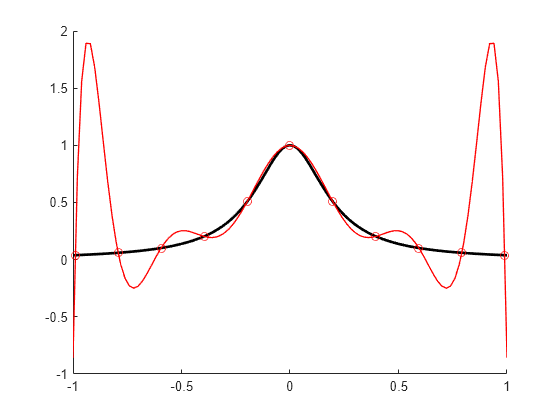
Plot runge, sp_es, and the interpolation points on the interval [-1 1].

figure
hold on
fplot(runge,[-1 1],"k",LineWidth=2);
plot(x_es,y_es,"ro")
fnplt(sp_es,[-1 1],"r",1)

The plot shows that sp_es has large oscillations near the interval boundaries.

To improve the fit, use chbpnt to find Chebyshev-Demko interpolation points for a Chebyshev spline of order 10 with knot sequence t.

x_cd = chbpnt(t,k);
y_cd = runge(x_cd);

Fit a spline to the Chebyshev-Demko interpolation points using the knot sequence t.

sp_cd = spapi(t,x_cd,y_cd)

sp_cd = struct with fields:
      form: 'B-'
     knots: [-1 -1 -1 -1 -1 -1 -1 -1 -1 -1 -1 1 1 1 1 1 1 1 1 1 1 1]
     coefs: [0.0385 0.2641 -2.5533 12.9011 -32.4456 46.7434 -32.4456 12.9011 -2.5533 0.2641 0.0385]
    number: 11
     order: 11
       dim: 1

sq_cd contains the results of the fit for the Chebyshev-Demko interpolation points.

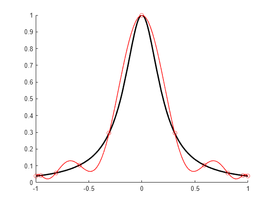
Plot runge, sp_cd, and the interpolation points on the interval [-1 1].

figure
hold on
fplot(runge,[-1 1],"k",LineWidth=2);
plot(x_cd,y_cd,"ro")
fnplt(sp_cd,[-1 1],"r",1)

The plot shows that sp_cd does not oscillate as much as sp_eq. sp_cd is a better approximation to runge near the interval boundaries.

To compare the accuracy of the splines, evaluate runge at 1000 equally spaced points in the interval [-1 1]. Use fnval to evaluate sp_es and sp_cd at the same points.

i = linspace(-1,1,1000);
runge_val = runge(i);
sp_es_val = fnval(sp_es,i);
sp_cd_val = fnval(sp_cd,i);

Calculate the sum of squares error (SSE) for sp_es and sp_cd using the function norm.

error_es = sp_es_val - runge_val;
error_cd = sp_cd_val - runge_val;

[norm(error_es)^2 norm(error_cd)^2]

ans = 1×2

  324.0260    3.8479

The smaller SSE for sp_cd shows that the Chebyshev-Demko interpolation points yield a better overall approximation for runge than the equally spaced interpolation points.

Algorithms

The Chebyshev spline for the given knot sequence and order is constructed iteratively, using the Remez algorithm, using as initial guess the spline that takes alternately the values 1 and −1 at the sequence aveknt(t,k). The example Construct Chebyshev Spline gives a detailed discussion of one version of the process as applied to a particular example.