The B-form
Introduction to B-form
A univariate spline f is specified by its nondecreasing
knot sequence t and by its B-spline coefficient sequence
a. See Multivariate Tensor Product Splines for a discussion
of multivariate splines. The coefficients may be (column-)vectors, matrices, even
ND-arrays. When the coefficients are 2-vectors or 3-vectors, f is a curve in
R2 or R3 and the coefficients are
called the
control points for the curve.
Roughly speaking, such a spline is a piecewise-polynomial of a certain order and with
breaks t(i). But knots are different from breaks in that they may be repeated, i.e., t need not be
strictly increasing. The resulting knot
multiplicities govern the smoothness of the spline across the knots, as detailed below.
With [d,n] = size(a), and n+k = length(t), the
spline is of order
k. This means that its polynomial pieces have degree <
k. For example, a cubic spline is a spline of order 4
because it takes four coefficients to specify a cubic polynomial.
Definition of B-form
These four items, t, a, n, and k, make up the B-form of the spline f.
This means, explicitly, that
with Bi,k=B(·|t(i:i+k)) the ith B-spline of order k for
the given knot sequence t, i.e., the B-spline with knots
t(i),...,t(i+k). The basic interval of this B-form is the interval
[t(1)..t(n+k)]. It is the default interval over which a spline in
B-form is plotted by the command fnplt. Note that a spline in B-form
is zero outside its basic interval while, after conversion to ppform via
fn2fm, this is usually not the case because, outside its basic
interval, a piecewise-polynomial is defined by extension of its first or last polynomial piece. In particular, a function
in B-form may have jumps in value and/or one of its derivative not only across its interior knots, i.e., across t(i) with
t(1)<t(i)<t(n+k), but also across its end knots, t(1) and
t(n+k).
B-form and B-Splines
The building blocks for the B-form of a spline are the B-splines. A B-Spline of Order 4, and the Four Cubic Polynomials from Which It Is Made shows a picture of such a B-spline, the one
with the knot sequence [0 1.5 2.3 4 5], hence of order 4, together
with the polynomials whose pieces make up the B-spline. The information for that picture
could be generated by the command
To summarize: The B-spline with knots t(i)≤····≤
t(i+k) is positive on the interval (t(i)..t(i+k))and is zero outside that interval. It is piecewise-polynomial of order
k with breaks at the sites t(i),...,t(i+k). These knots may coincide, and the precise
multiplicity governs the smoothness with which the two
polynomial pieces join there.
Definition of B-Splines
The shorthand
is one of several ways to indicate that f is a spline of order
k with knot sequence t, i.e., a
linear combination of the B-splines of order k for
the knot sequence t.
A word of caution: The term B-spline has been expropriated by the Computer-Aided Geometric Design (CAGD) community to mean what is called here a spline in B-form, with the unhappy result that, in any discussion between mathematicians/approximation theorists and people in CAGD, one now always has to check in what sense the term is being used.
B-Spline Knot Multiplicity
The rule is
knot multiplicity + condition multiplicity = order
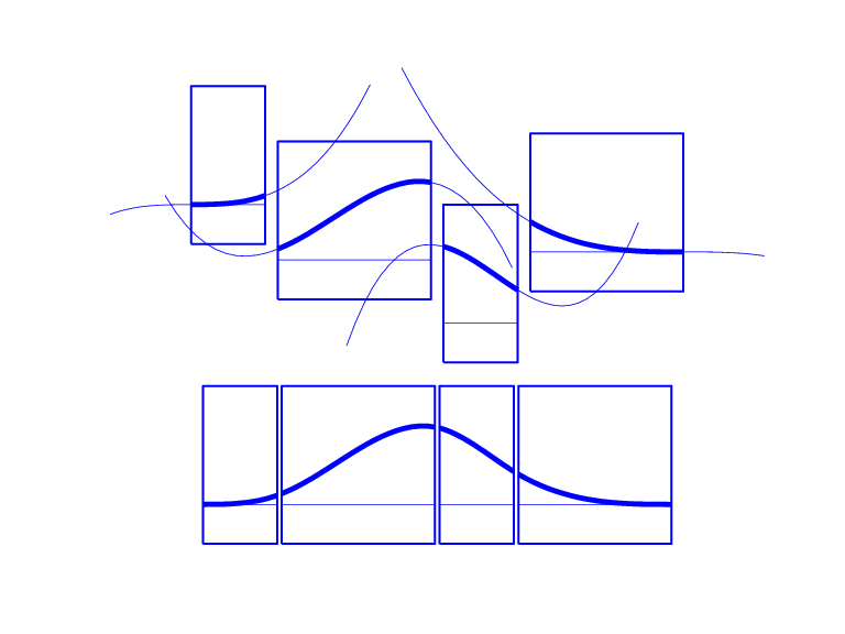
All Third-Order B-Splines for a Certain Knot Sequence with Various Knot Multiplicities

For example, for a B-spline of order 3, a simple knot would mean two smoothness conditions, i.e., continuity of function and first derivative, while a double knot would only leave one smoothness condition, i.e., just continuity, and a triple knot would leave no smoothness condition, i.e., even the function would be discontinuous.
All Third-Order B-Splines for a Certain Knot Sequence with Various Knot Multiplicities shows a picture of all the third-order B-splines for a certain mystery knot sequence
t. The breaks are indicated by vertical lines. For each break, try
to determine its multiplicity in the knot sequence (it is 1,2,1,1,3), as well as its
multiplicity as a knot in each of the B-splines. For example, the second break has
multiplicity 2 but appears only with multiplicity 1 in the third B-spline and not at
all, i.e., with multiplicity 0, in the last two B-splines. Note that only one of the
B-splines shown has all its knots simple. It is the only one having three different
nontrivial polynomial pieces. Note also that you can tell the knot-sequence multiplicity
of a knot by the number of B-splines whose nonzero part begins or ends there. The
picture is generated by the following MATLAB® statements, which use the command spcol from this toolbox to generate the function values of all
these B-splines at a fine net x.
t=[0,1,1,3,4,6,6,6]; x=linspace(-1,7,81);
c=spcol(t,3,x);[l,m]=size(c);
c=c+ones(l,1)*[0:m-1];
axis([-1 7 0 m]); hold on
for tt=t, plot([tt tt],[0 m],'-'), end
plot(x,c,'linew',2), hold off, axis off
Further illustrated examples are provided by the example ”Construct and Work
with the B-form”. You can also use the GUI bspligui to study
the dependence of a B-spline on its knots experimentally.
Choice of Knots for B-form
The rule “knot multiplicity + condition multiplicity = order” has the following consequence for the process of choosing a knot sequence for the B-form of a spline approximant. Suppose the spline s is to be of order k, with basic interval [a..b], and with interior breaks ξ2< ·· ·<ξl. Suppose, further, that, at ξi, the spline is to satisfy μi smoothness conditions, i.e.,
Then, the appropriate knot sequence t should contain the break ξi exactly k – μi times, i=2,...,l. In addition, it should contain the two endpoints, a and b, of the basic interval exactly k times. This last requirement can be relaxed, but has become standard. With this choice, there is exactly one way to write each spline s with the properties described as a weighted sum of the B-splines of order k with knots a segment of the knot sequence t. This is the reason for the B in B-spline: B-splines are, in Schoenberg's terminology, basic splines.
For example, if you want to generate the B-form of a cubic spline on the interval [1 .. 3], with interior breaks 1.5, 1.8, 2.6, and with two continuous derivatives, then the following would be the appropriate knot sequence:
t = [1, 1, 1, 1, 1.5, 1.8, 2.6, 3, 3, 3, 3];
This is supplied by augknt([1, 1.5, 1.8, 2.6, 3], 4). If you
wanted, instead, to allow for a corner at 1.8, i.e., a possible jump in the first derivative there, you would triple the knot 1.8, i.e.,
use
t = [1, 1, 1, 1, 1.5, 1.8, 1.8, 1.8, 2.6, 3, 3, 3, 3];
and this is provided by the statement
t = augknt([1, 1.5, 1.8, 2.6, 3], 4, [1, 3, 1] );