ifir

Interpolated FIR filter design

Syntax

[h,g] = ifir(l,type,f,dev)
[h,g,d] = ifir(l,type,f,dev)
[...] = ifir(...,str)


Description

[h,g] = ifir(l,type,f,dev) designs a periodic filter h(zl), where l is the interpolation factor. It also finds an image-suppressor filter g(z), such that the cascade of the two filters represents the optimal minimax FIR approximation of the desired response. This response is specified by type, with band edge frequencies contained in vector f. This is done while not exceeding the maximum deviations or ripples (linear) specified in vector dev.

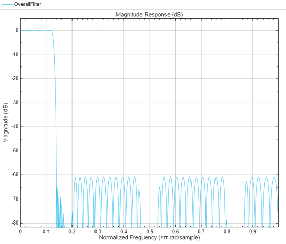
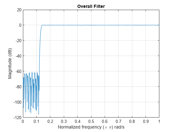
When type is set to 'low', the filter design is a lowpass design. When type is set to 'high', the filter design is a highpass design. f is a two-element vector with passband and stopband edge frequency values. For narrowband lowpass filters and wideband highpass filters, l×f(2) is less than 1. For wideband lowpass filters and narrowband highpass filters, specify f so that l×(1–f(1)) is less than 1.

dev is a two-element vector that contains the peak ripple or deviation (in linear units) allowed for both the passband and the stopband.

The ifir design algorithm achieves an efficient design in the sense that it reduces the total number of multipliers required. To do this, the design problem is broken into two stages. In the first stage, the filter is upsampled to achieve the stringent specifications without using many multipliers. In the second stage, the filter removes the images created when upsampling the previous filter.

[h,g,d] = ifir(l,type,f,dev) returns a delay d that is connected in parallel with the cascade of h(zl) and g(z) for both wideband lowpass and highpass filters. This is necessary to obtain the desired response.

[...] = ifir(...,str) uses str to choose the algorithm level of optimization used. Possible values for str are 'simple', 'intermediate' (default) or 'advanced'. str provides for a tradeoff between design speed and filter order optimization. The 'advanced' option can result in substantial filter order reduction, especially for g(z).

Examples

Narrowband lowpass design using an interpolation factor of 6

This example shows how to use the function ifir to design a narrowband lowpass filter.

[h,g] = ifir(6,'low',[.12 .14],[.01 .001]);
H = dsp.FIRFilter(Numerator=h);
G = dsp.FIRFilter(Numerator=g);
filterAnalyzer(H,G,FilterNames=["PeriodicFilter","ImageSuppressorFilter"]);

Hcas = cascade(H,G);
filterAnalyzer(Hcas,FilterNames="OverallFilter");

Wideband highpass design using an interpolation factor of 6

This example shows how to use ifir to design a wideband highpass filter.

[h,g,d]=ifir(6,'high',[.12 .14],[.001 .01]);
H = dsp.FIRFilter('Numerator',h); G = dsp.FIRFilter('Numerator',g);
b1 = cascade(H,G);                 % Branch 1
b2 = dsp.FIRFilter('Numerator',d); % Branch 2
Hoverall = freqz(b1) + freqz(b2); % Overall wideband highpass
plot(linspace(0,1,length(Hoverall)),20*log10(abs(Hoverall)))
xlabel('Normalized frequency (\times \pi) rad/s')
ylabel('Magnitude (dB)')
title('Overall Filter');
grid on

Design a cascade of lowpass filters

This example shows how to use fdesign.lowpass to design a cascade of lowpass filters. After designing the filter, plot the response curve.

fpass = 0.2;
fstop = 0.24;
d1 = fdesign.lowpass(fpass, fstop);
lowpassCascade = design(d1,'ifir',Systemobject=true);
filterAnalyzer(lowpassCascade)

Extended Capabilities

C/C++ Code Generation

Generate C and C++ code using MATLAB® Coder™.

Usage notes and limitations:

All inputs must be constant. Expressions or variables are allowed if their values do not change.

Version History

Introduced in R2011a