Tasking Modes and Execution Order
The tasking mode that Simulink® uses when scheduling the tasks associated with a model depends on the setting of the model configuration parameter Treat each discrete rate as a separate task. When cleared, the parameter specifies single-tasking mode. When selected, the parameter specifies multitasking mode.
| Tasking Mode | Scheduling Behavior |
|---|---|
| Single-tasking mode | The blocks that are in a model execute as one task. Simulink determines the block execution order during a model update. |
| Multitasking mode | Simulink groups the blocks that are in a model based on the block sample time. For example, if a model includes blocks that use sample time 0.1 or 1, Simulink places the blocks that use the fastest sample time 0.1 in task 0 and blocks that use sample time 1 in task 1. Simulink determines the block execution order during a model update. |
Single-Tasking Execution
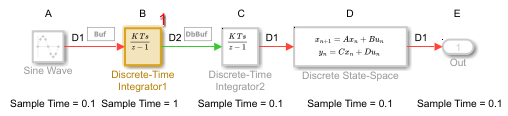
Consider this multirate model, which is configured for single-tasking execution.
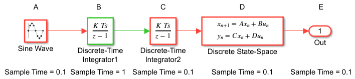
The letters A to E identify the blocks in timing diagrams that appear in subsections below.
To view the execution order of the blocks in the model, from the model window toolstrip, select Debug > Information Overlays > Execution Order.
This figure shows the execution order of the preceding model.
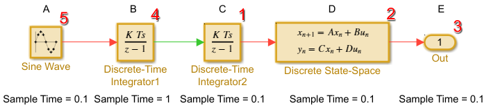
The numbers that appear above the top right corner of the blocks indicate the execution order.
This table shows the block execution order and for each block the sample time and whether the block has output and update computations.
Blocks | Sample Time | Output Computation | Update Computation |
|---|---|---|---|
C | 0.1 | Y | Y |
D | 0.1 | Y | Y |
E | 0.1 | N | N |
B | 1 | Y | Y |
A | 0.1 | Y | N |
For more information, see Simulation Phases in Dynamic Systems.
Simulated Single-Tasking Execution
This timing diagram shows the execution of the model during a Simulink simulation loop. During simulation, execution time is assumed to be zero.
Because time is simulated, the placement of ticks represents the iterations of the simulation loop. During simulation, Idle time is not present between simulated sample periods.
Real-Time Single-Tasking Execution
In a real-time system, the execution order determines the order in which blocks execute within a given time interval or task. This figure shows the scheduling of computations when the generated code is deployed in single-tasking mode within a real-time system. The generated program runs in real time under control of interrupts from a 10 Hz timer.
Blocks execute in the same order as in the figure for simulation, but with the constraint of a real-time clock.
At times 0.0, 1.0, and every second thereafter, the slow and fast blocks execute output computations followed by update computations for blocks that have states. Within a given time interval, output and update computations are sequenced in block execution order.
The fast blocks execute on every tick, at intervals of 0.1 second. The slow blocks execute 10 ticks, at intervals of 1 second. Output computations are followed by update computations.
The system spends some portion of each time interval (labeled “wait”) idling. During the intervals when only the fast blocks execute, a larger portion of the interval is spent idling. This illustrates an inherent inefficiency of single-tasking mode.
Multitasking Execution
Consider the same model shown in Single-Tasking Execution, but configured for multitasking execution.
The letters A to E identify the blocks in timing diagrams that appear in subsections below.
Because rate transitions occur in the model, this version of the model has the solver
model configuration parameter Automatically handle rate transitions for
data selected and parameter Deterministic data
transfer set to Whenever possible (the
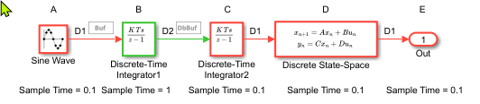
default).The buffer (Buf) and double buffer (DbBuf) symbols identify where Simulink inserts hidden Rate Transition blocks.
To view the execution order of the blocks associated with each task in the model, from the model window toolstrip, select Debug > Information Overlays > Execution Order. Then, near the bottom of the Execution Order pane, select Task 0 or Task 1 to display the execution order of that task.
This figure shows the execution order for task 0 (sample time = 0.1) of the model.
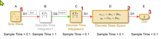
This table shows the execution order for blocks grouped in task 0 and whether a block has output and update computations.
Blocks | Output Computation | Update Computation |
|---|---|---|
C | Y | Y |
D | Y | Y |
E | Y | N |
A | Y | N |
This figure shows the execution order for task 1 (sample time = 1) of the model.
This table shows the execution order for blocks grouped in task 1 and whether a block has output and update computations.
Blocks | Output Computation | Update Computation |
|---|---|---|
B | Y | Y |
Note
The timing diagrams in the following subsections assume that the Rate Transition blocks use the default (protected) mode, with block parameters Ensure data integrity during data transfer and Ensure deterministic data transfer (maximum delay) selected.
Simulated Multitasking Execution
This figure shows a simulation of the model in multitasking mode. The Simulink engine assumes zero execution time for the blocks, eliminating the need for preemption.
Real-Time Multitasking Execution
This figure shows the scheduling of computations when the generated code is deployed in a real-time system in multitasking mode. The generated program runs in real time as two tasks under control of interrupts from a 10 Hz (fast) and 1 Hz (slow) timers. Preemption can occur. For example, if task 0 becomes active while block B in task 1 is computing output, task 0 preempts task 1.
if the output computation of block B in task1takes a long time and task 0 becomes active again before the output computation of B finishes.