Plot a Confidence Band Using HAC Estimates
This example shows how to plot heteroscedastic-and-autocorrelation consistent (HAC) corrected confidence bands using Newey-West robust standard errors.
One way to estimate the coefficients of a linear model is by OLS. However, time series models tend to have innovations that are autocorrelated and heteroscedastic (i.e., the errors are nonspherical). If a time series model has nonspherical errors, then usual formulae for standard errors of OLS coefficients are biased and inconsistent. Inference based on these inefficient standard errors tends to inflate the Type I error rate. One way to account for nonspherical errors is to use HAC standard errors. In particular, the Newey-West estimator of the OLS coefficient covariance is relatively robust against nonspherical errors.
Load Data
Load the Canadian electric power consumption data set from the World Bank. The response is Canada's electrical energy consumption in kWh (DataTimeTable.consump), the predictor is Canada's GDP in year 2000 USD (DataTimeTable.gdp), and the data set also contains the GDP deflator (DataTimeTable.gdp_deflator). Because DataTimeTable is a timetable, DataTimeTable.Time is the sample year.
load Data_PowerConsumptionDefine Model
Model the behavior of the annual difference in electrical energy consumption with respect to real GDP as a linear model:
consumpDiff = diff(DataTimeTable.consump);  % Annual difference in consumption
consumpDiff = consumpDiff/1.0e+10;          % Scale for numerical stability
T = size(consumpDiff,1);

rGDP = DataTimeTable.gdp./(DataTimeTable.gdp_deflator); % Deflate GDP
rGDP = rGDP(2:end)/1.0e+10;

Mdl = fitlm(rGDP,consumpDiff);
coeff = Mdl.Coefficients(:,1);
EstParamCov = Mdl.CoefficientCovariance;
resid = Mdl.Residuals.Raw;
Plot Data
Plot the difference in energy consumption, consumpDiff versus the real GDP, to check for possible heteroscedasticity.
figure
plot(rGDP,consumpDiff,".")
title("Annual Difference in Energy Consumption vs real GDP - Canada")
xlabel("Real GDP (year 2000 USD)")
ylabel("Annual Difference in Energy Consumption (kWh)")
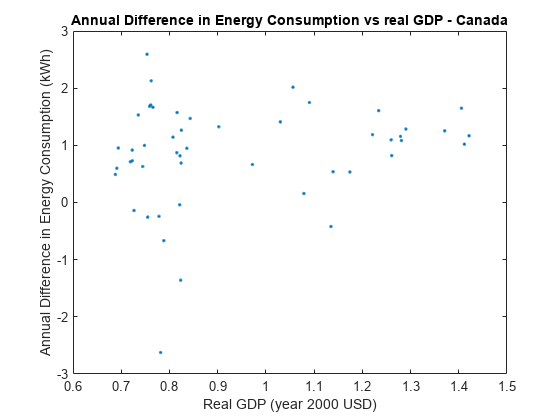
The figure indicates that heteroscedasticity might be present in the annual difference in energy consumption. As real GDP increases, the annual difference in energy consumption seems to be less variable.
Plot Residuals
Plot the residuals from Mdl against the fitted values and year to assess heteroscedasticity and autocorrelation.
figure
tiledlayout("flow")
nexttile([1 2])
plot(Mdl.Fitted,resid,".")
hold on
plot([min(Mdl.Fitted) max(Mdl.Fitted)],[0 0],"k-")
title("Residual Plots")
xlabel("Fitted Consumption")
ylabel("Residuals")
axis tight
hold off
nexttile
autocorr(resid)
h1 = gca;
h1.FontSize = 8;
nexttile
parcorr(resid)
h2 = gca;
h2.FontSize = 8;
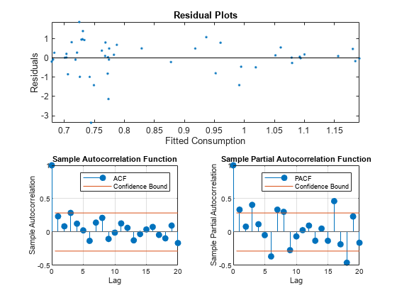
The residual plot reveals decreasing residual variance with increasing fitted consumption. The autocorrelation function shows that autocorrelation might be present in the first few lagged residuals.
Test for Heteroscedasticity and Autocorrelation
Test for conditional heteroscedasticity using Engle's ARCH test. Test for autocorrelation using the Ljung-Box Q test. Test for overall correlation using the Durbin-Watson test.
[~,englePValue] = archtest(resid);
englePValue
englePValue =
0.1463
[~,lbqPValue] = lbqtest(resid,Lag=1:3); % Significance of first three lags
lbqPValue
lbqPValue = 1×3
0.0905 0.1966 0.0522
[dwPValue] = dwtest(Mdl);
dwPValue
dwPValue =
0.0024
The p value of Engle's ARCH test suggests significant conditional heteroscedasticity at 15% significance level. The p value for the Ljung-Box Q test suggests significant autocorrelation with the first and third lagged residuals at 10% significance level. The p value for the Durbin-Watson test suggests that there is strong evidence for overall residual autocorrelation. The results of the tests suggest that the standard linear model conditions of homoscedasticity and uncorrelated errors are violated, and inferences based on the OLS coefficient covariance matrix are suspect.
One way to proceed with inference (such as constructing a confidence band) is to correct the OLS coefficient covariance matrix by estimating the Newey-West coefficient covariance.
Estimate Newey-West Coefficient Covariance
Correct the OLS coefficient covariance matrix by estimating the Newey-West coefficient covariance using hac. Compute the maximum lag to be weighted for the standard Newey-West estimate, maxLag (Newey and West, 1994). Use hac to estimate the standard Newey-West coefficient covariance.
maxLag = floor(4*(T/100)^(2/9));
[NWEstParamCov,~,NWCoeff] = hac(Mdl,Type="HAC", ...
    Bandwidth=maxLag+1);
Estimator type: HAC
Estimation method: BT
Bandwidth: 4.0000
Whitening order: 0
Effective sample size: 49
Small sample correction: on

Coefficient Covariances:

       |  Const      x1
--------------------------
 Const |  0.3720  -0.2990
 x1    | -0.2990   0.2454
The Newey-West standard error for the coefficient of rGDP, labeled in the table, is less than the usual OLS standard error. This suggests that, in this data set, correcting for residual heteroscedasticity and autocorrelation increases the precision in measuring the linear effect of real GDP on energy consumption.
Calculate Working-Hotelling Confidence Bands
Compute the 95% Working-Hotelling confidence band for each covariance estimate using nlpredci (Kutner et al., 2005).
rGDPdes = [ones(T,1) rGDP];                         % Design matrix
modelfun = @(b,x)(b(1)*x(:,1)+b(2)*x(:,2));         % Define the linear model

[beta,nlresid,~,EstParamCov] = nlinfit(rGDPdes, ...
    consumpDiff,modelfun,[1,1]);                    % Estimate the model

[fity,fitcb] = nlpredci(modelfun,rGDPdes,beta,nlresid, ...
    Covar=EstParamCov,SimOpt="on");                 % Margin of errors
conbandnl = [fity - fitcb fity + fitcb];            % Confidence bands
[fity,NWfitcb] = nlpredci(modelfun,rGDPdes, ...
    beta,nlresid,Covar=NWEstParamCov,SimOpt="on");  % Corrected margin of error
NWconbandnl = [fity - NWfitcb fity + NWfitcb];      % Corrected confidence bands
Plot Working-Hotelling Confidence Bands
Plot the Working-Hotelling confidence bands on the same axes twice: one plot displaying electrical energy consumption with respect to real GDP, and the other displaying the electrical energy consumption time series.
figure
l1 = plot(rGDP,consumpDiff,"k.");
hold on
l2 = plot(rGDP,fity,"b-",LineWidth=2);
l3 = plot(rGDP,conbandnl,"r-");
l4 = plot(rGDP,NWconbandnl,"g--");
title("Data with 95% Working-Hotelling Conf. Bands")
xlabel("real GDP (year 2000 USD)")
ylabel("Consumption (kWh)")
axis([0.7 1.4 -2 2.5])
legend([l1 l2 l3(1) l4(1)],"Data","Fitted","95% conf. band", ...
    "Newey-West 95% conf. band",Location="southeast")
hold off
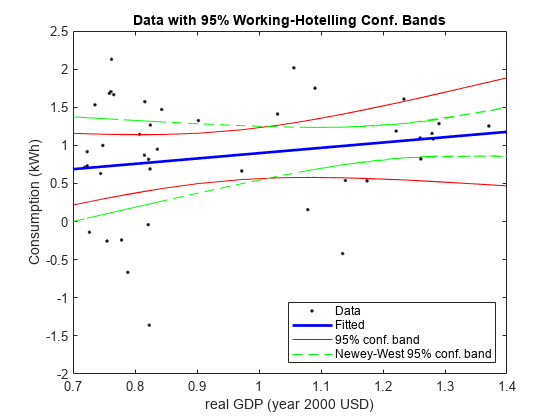
figure
year = DataTimeTable.Time(2:end);
l1 = plot(year,consumpDiff);
hold on
l2 = plot(year,fity,"k-",LineWidth=2);
l3 = plot(year,conbandnl,"r-");
l4 = plot(year,NWconbandnl,"g--");
title("Consumption with 95% Working-Hotelling Conf. Bands")
xlabel("Year")
ylabel("Consumption (kWh)")
legend([l1 l2 l3(1) l4(1)],"Consumption","Fitted", ...
    "95% conf. band","Newey-West 95% conf. band", ...
    Location="southwest")
hold off
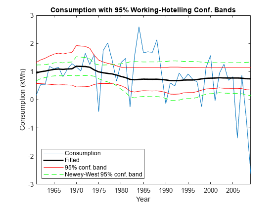
The plots show that the Newey-West estimator accounts for the heteroscedasticity in that the confidence band is wide in areas of high volatility, and thin in areas of low volatility. The OLS coefficient covariance estimator ignores this pattern of volatility.
References:
Kutner, M. H., C. J. Nachtsheim, J. Neter, and W. Li. Applied Linear Statistical Models. 5th Ed. New York: McGraw-Hill/Irwin, 2005.
Newey, W. K., and K. D. West. "A Simple Positive Semidefinite, Heteroskedasticity and Autocorrelation Consistent Covariance Matrix." Econometrica. Vol. 55, 1987, pp. 703-708.
Newey, W. K, and K. D. West. "Automatic Lag Selection in Covariance Matrix Estimation." The Review of Economic Studies. Vol. 61 No. 4, 1994, pp. 631-653.