forecast
Forecast sample paths from threshold-switching dynamic regression model
Since R2021b
Syntax
Description
YF = forecast(Mdl,Y,numPeriods)YF of a fully specified
threshold-switching dynamic regression model Mdl over a forecast
horizon of length numPeriods. The forecasted responses represent the
continuation of the response data Y.
YF = forecast(Mdl,Y,numPeriods,Name,Value)forecast(Mdl,Y,10,Type="exogenous",Z=z)
specifies exogenous-type forecasts and forecast-period, exogenous threshold variable data
z.
Examples
This example shows how to compute iterative point forecasts of the conditional mean of a self-exciting threshold autoregressive (SETAR) model. Specify all parameter values (this example uses arbitrary values).
Create Fully Specified Model for DGP
Create a discrete threshold transition at level 0.
t = 0;
tt = threshold(t)
tt =
  threshold with properties:

          Type: 'discrete'
        Levels: 0
         Rates: []
    StateNames: ["1"    "2"]
     NumStates: 2
tt is a fully specified threshold object that describes the switching mechanism of the threshold-switching model.
Assume the following univariate models describe the response process of the system:
State 1: .
State 2: .
.
For each regime, use arima to create an AR model that describes the response process within the regime.
c1 = -1;
c2 = 1;
ar = 0.6;

mdl1 = arima(Constant=c1,AR=ar)
mdl1 =
  arima with properties:

     Description: "ARIMA(1,0,0) Model (Gaussian Distribution)"
      SeriesName: "Y"
    Distribution: Name = "Gaussian"
               P: 1
               D: 0
               Q: 0
        Constant: -1
              AR: {0.6} at lag [1]
             SAR: {}
              MA: {}
             SMA: {}
     Seasonality: 0
            Beta: [1×0]
        Variance: NaN
mdl2 = arima(Constant=c2,AR=ar)
mdl2 =
  arima with properties:

     Description: "ARIMA(1,0,0) Model (Gaussian Distribution)"
      SeriesName: "Y"
    Distribution: Name = "Gaussian"
               P: 1
               D: 0
               Q: 0
        Constant: 1
              AR: {0.6} at lag [1]
             SAR: {}
              MA: {}
             SMA: {}
     Seasonality: 0
            Beta: [1×0]
        Variance: NaN
mdl1 and mdl2 are effectively, fully specified arima objects. The innovations variances of the submodels are unspecified; the tsVAR object specifies the model-wide innovations variance.
Store the submodels in a vector with order corresponding to the regimes in tt.StateNames.
mdl = [mdl1; mdl2];
Use tsVAR to create a TAR model from the switching mechanism tt and the state-specific submodels mdl. Specify a model-wide innovations variance of 0.5.
Mdl = tsVAR(tt,mdl,Covariance=0.5)
Mdl =
  tsVAR with properties:

         Switch: [1×1 threshold]
      Submodels: [2×1 varm]
      NumStates: 2
      NumSeries: 1
     StateNames: ["1"    "2"]
    SeriesNames: "1"
     Covariance: 0.5000
Mdl.Submodels(2)
ans =
  varm with properties:

     Description: "AR-Stationary 1-Dimensional VAR(1) Model"
     SeriesNames: "Y1"
       NumSeries: 1
               P: 1
        Constant: 1
              AR: {0.6} at lag [1]
           Trend: 0
            Beta: [1×0 matrix]
      Covariance: NaN
Mdl is a fully specified tsVAR object representing a univariate two-state TAR model. tsVAR stores specified arima submodels as varm objects.
Simulate Response Data from DGP
forecast requires enough data before the forecast horizon to initialize the model. Simulate 120 observations from the DGP.
rng(1); % For reproducibility
y = simulate(Mdl,120);
y is a 120-by-1 random path of responses. The default options of simulate, and all tsVAR object functions, specify that the threshold variable is .
Compute Optimal Point Forecasts
Treat the first 100 observations of the simulated response data as the presample for the forecast, and treat the last 10 observations as a holdout sample.
idx0 = 1:100;
idx1 = 101:120;
y0 = y(idx0);
y1 = y(idx1);
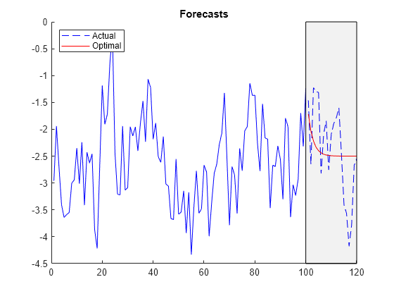
Compute 1- through 20-step-ahead optimal point forecasts from the model.
yf = forecast(Mdl,y0,20);
yf is a 20-by-1 vector of optimal point forecasts.
Plot the simulated response data and forecasts.
figure
hold on
plot(idx0,y0,'b');
h = plot(idx1,y1,'b--');
h1 = plot(idx1,yf,'r');
yfill = [ylim fliplr(ylim)];
xfill = [idx0(end) idx0(end) idx1(end) idx1(end)];
fill(xfill,yfill,'k','FaceAlpha',0.05)
legend([h h1],["Actual" "Optimal"],'Location','NorthWest')
title('Forecasts')
hold off
forecast must use Monte Carlo methods to estimate forecast error variances. Therefore, when simulate returns forecast error variances, it uses Monte Carlo methods to compute point forecasts.
Create the SETAR model in Compute Optimal Point Forecasts.
t = 0;
tt = threshold(t);
c1 = -1;
c2 = 1;
ar = 0.6;
mdl1 = arima(Constant=c1,AR=ar);
mdl2 = arima(Constant=c2,AR=ar);
mdl = [mdl1; mdl2];

Mdl = tsVAR(tt,mdl,Covariance=0.5);
forecast requires enough data before the forecast horizon to initialize the model. Simulate 120 observations from the DGP.
rng(100); % For reproducibility
fh = 20;
y = simulate(Mdl,100+fh);
Treat the first 100 observations of the simulated response data as the presample for the forecast, and treat the last 20 observations as a holdout sample.
idx0 = 1:100;
idx1 = 101:(100 + fh);
y0 = y(idx0);
y1 = y(idx1);
Compute 1- through 20-step-ahead optimal point forecasts from the model.
yf1 = forecast(Mdl,y0,fh);
yf1 is a 20-by-1 vector of optimal point forecasts.
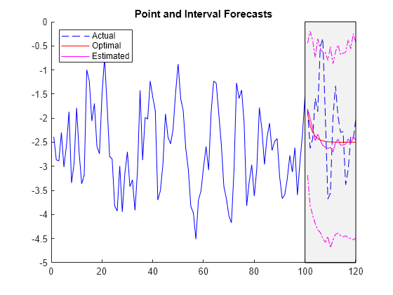
Compute 1- through 20-step-ahead Monte Carlo point forecasts by returning the estimated forecast error variances.
[yf2,estVar] = forecast(Mdl,y0,fh);
yf2 is a 20-by-1 vector of Monte Carlo point forecasts. estVAR is a 20-by-1 vector of corresponding estimated forecast error variances.
Plot the simulated response data, forecasts, and 95% forecast intervals using the Monte Carlo estimates.
figure
hold on
plot(idx0,y0,'b');
h = plot(idx1,y1,'b--');
h1 = plot(idx1,yf1,'r');
h2 = plot(idx1,yf2,'m');
ciu = yf2 + 1.96*sqrt(estVar); % Upper 95% confidence level
cil = yf2 - 1.96*sqrt(estVar); % Lower 95% confidence level
plot(idx1,ciu,'m-.');
plot(idx1,cil,'m-.');
yfill = [ylim,fliplr(ylim)];
xfill = [idx0(end) idx0(end) idx1(end) idx1(end)];
fill(xfill,yfill,'k','FaceAlpha',0.05)
legend([h h1 h2],["Actual" "Optimal" "Estimated"],...
    'Location',"NorthWest")
title("Point and Interval Forecasts")
hold off
When forecast performs Monte Carlo methods to estimate point forecasts and forecast error covariances, you can adjust the number of paths to sample by specifying the NumPaths option.
Create the SETAR model in Compute Optimal Point Forecasts.
t = 0;
tt = threshold(t);
c1 = -1;
c2 = 1;
ar = 0.6;
mdl1 = arima(Constant=c1,AR=ar);
mdl2 = arima(Constant=c2,AR=ar);
mdl = [mdl1; mdl2];

Mdl = tsVAR(tt,mdl,Covariance=0.5);
forecast requires enough data before the forecast horizon to initialize the model. Simulate 120 observations from the DGP.
rng(100); % For reproducibility
fh = 20;
y = simulate(Mdl,100+fh);
Treat the first 100 observations of the simulated response data as the presample for the forecast, and treat the last 20 observations as a holdout sample.
idx0 = 1:100;
idx1 = 101:(100 + fh);
y0 = y(idx0);
y1 = y(idx1);
Compute 1- through 20-step-ahead optimal point forecasts from the model.
yf1 = forecast(Mdl,y0,fh);
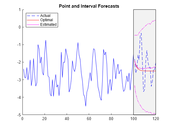
Compute 1- through 20-step-ahead Monte Carlo point forecasts by returning the estimated forecast error variances. Specify a Monte Carlo sample of 1000 paths.
[yf2,estVar] = forecast(Mdl,y0,fh,NumPaths=1000);
yf2 is a 20-by-1 vector of Monte Carlo point forecasts. estVAR is a 20-by-1 vector of corresponding estimated forecast error variances.
Plot the simulated response data, forecasts, and 95% forecast intervals using the Monte Carlo estimates.
figure
hold on
plot(idx0,y0,'b');
h = plot(idx1,y1,'b--');
h1 = plot(idx1,yf1,'r');
h2 = plot(idx1,yf2,'m');
ciu = yf2 + 1.96*sqrt(estVar); % Upper 95% confidence level
cil = yf2 - 1.96*sqrt(estVar); % Lower 95% confidence level
plot(idx1,ciu,'m-.');
plot(idx1,cil,'m-.');
yfill = [ylim,fliplr(ylim)];
xfill = [idx0(end) idx0(end) idx1(end) idx1(end)];
fill(xfill,yfill,'k',FaceAlpha=0.05)
legend([h h1 h2],["Actual" "Optimal" "Estimated"],Location="NorthWest")
title("Point and Interval Forecasts")
hold off
Consider a logistic threshold-switching model (LSTAR) for the real US GDP growth rate, where each submodel is AR(4) and the threshold variable is the unemployment growth rate.
Create a partially specified threshold transition for the unemployment growth rate. Specify the logistic transition function, and an unknown, estimable mid-level and rate. Label the states "Contraction" and "Expansion".
tt = threshold(NaN,Type="logistic",Rates=NaN,...
    StateNames=["Contraction" "Expansion"]);
tt is a partially specified threshold object, and it is agnostic of the variable and data it represents.
Create a threshold-switching model for the real US GDP growth rate.
p = 4;
mdl = [arima(ARLags=p); arima(ARLags=p)];
Mdl = tsVAR(tt,mdl);
Mdl is a partially specified tsVAR object specifying the structure of the model and which parameters are estimable.
Load the quarterly US macroeconomic data set Data_USEconModel. Remove leading missing values in the series. Compute the real GDP percent growth and unemployment growth.
load Data_USEconModel
DataTimeTable = rmmissing(DataTimeTable,DataVariables=["GDP" "GDPDEF" "UNRATE"]);
RGDP = DataTimeTable.GDP./DataTimeTable.GDPDEF;
rRGDP = price2ret(RGDP);            % Response data
gUNRATE = diff(DataTimeTable.UNRATE);   % Exogenous threshold data
dts = DataTimeTable.Time(2:end);
T = numel(dts);
Hold out the following sets from estimation:
The first four observations as a presample for estimation.
The final 25% as a forecast horizon to compare with the forecasts.
fh = ceil(0.25*T);
idxPre = 1:p;
idxEst = (idxPre(end)+1):(T-fh);
idxF = (T-fh+1):T;
To initialize the estimation procedure, fully specify a threshold transition that has the same structure as tt, but set the mid-level to 0 and a rate of 1 (the default).
tt0 = threshold(0,Type=tt.Type);
Fit the LSTAR model to the estimation period of the US GDP growth rate series. Specify the following parameters:
Set
Y0to the responses before the estimation period to initialize the AR submodel components.Set
Typeto"exogenous"to characterize the threshold variable.Set
Zto the threshold variable datagUNRATEin the estimation period.
EstMdl = estimate(Mdl,tt0,rRGDP(idxEst),Y0=rRGDP(idxPre), ...
    Type="exogenous",Z=gUNRATE(idxEst));
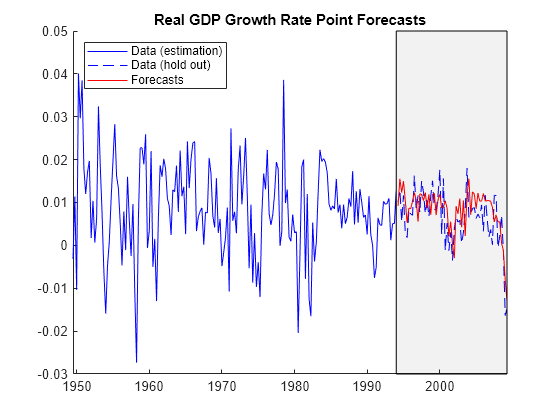
Forecast the real GDP growth rate series into the forecast horizon. Initialize the forecasts by specifying all responses in the estimation period (forecast uses only the latest, required observations). Characterize the threshold variable and provide its data in the forecast horizon.
yF = forecast(EstMdl,rRGDP(idxEst),fh,Type="exogenous",Z=gUNRATE(idxF));Plot the real GDP growth rate series with the forecasts.
figure
hold on
h1 = plot(dts(idxEst),rRGDP(idxEst),'b');
h2 = plot(dts(idxF),rRGDP(idxF),'b--');
h3 = plot(dts(idxF),yF,'r');
yfill = [ylim,fliplr(ylim)];
xfill = dts([idxEst(end) idxEst(end) idxF(end) idxF(end)]);
fill(xfill,yfill,'k',FaceAlpha=0.05)
legend([h1 h2 h3],["Data (estimation)" "Data (hold out)" "Forecasts"],...
    Location="NorthWest")
title("Real GDP Growth Rate Point Forecasts")
hold off
Consider the following 2-D LSETAR model.
State 1,
"Low": whereState 2 ,
"Med": whereState 3,
"High": whereThe system is in state 1 when , the system is in state 2 when , and the system is in state 3 otherwise.
The transition function is logistic. The transition rate from state 1 to 2 is 3.5, and the transition rate from state 1 to 3 is 1.5.
Create logistic threshold transitions at mid-levels -1 and 1 with rates 3.5 and 1.5, respectively. Label the states.
t = [-1 1];
r = [3.5 1.5];
stateNames = ["Low" "Med" "High"];
tt = threshold(t,Type="logistic",Rates=[3.5 1.5],StateNames=stateNames);
Create the VAR submodels by using varm. Store the submodels in a vector with order corresponding to the regimes in tt.StateNames.
% Constants (numSeries x 1 vectors)
C1 = [1; -1];
C2 = [2; -2];
C3 = [3; -3];

% Autoregression coefficients (numSeries x numSeries matrices)
AR1 = {};                            % 0 lags
AR2 = {[0.5 0.1; 0.5 0.5]};          % 1 lag
AR3 = {[0.25 0; 0 0] [0 0; 0.25 0]}; % 2 lags

% Innovations covariances (numSeries x numSeries matrices)
Sigma1 = [1 -0.1; -0.1 1];
Sigma2 = [2 -0.2; -0.2 2];
Sigma3 = [3 -0.3; -0.3 3];

% VAR Submodels
mdl1 = varm('Constant',C1,'AR',AR1,'Covariance',Sigma1);
mdl2 = varm('Constant',C2,'AR',AR2,'Covariance',Sigma2);
mdl3 = varm('Constant',C3,'AR',AR3,'Covariance',Sigma3);

mdl = [mdl1; mdl2; mdl3];
Create an LSETAR model from the switching mechanism tt and the state-specific submodels mdl. Label the series Y1 and Y2.
Mdl = tsVAR(tt,mdl,SeriesNames=["Y1" "Y2"])
Mdl =
  tsVAR with properties:

         Switch: [1×1 threshold]
      Submodels: [3×1 varm]
      NumStates: 3
      NumSeries: 2
     StateNames: ["Low"    "Med"    "High"]
    SeriesNames: ["Y1"    "Y2"]
     Covariance: []
Mdl is a fully specified tsVAR object representing a multivariate three-state LSETAR model. tsVAR object functions enable you to specify threshold variable characteristics and data.
Simulate Responses for Forecast Presample
You must specify enough presample observations to initialize all AR components in the VAR models and the endogenous threshold variable. The largest AR component order is 2 and the threshold variable delay is 4. Therefore, simulate and forecast require four presample observations per series and path.
Simulate one 2-D path of 100 observations from the model. Specify the endogenous threshold variable and its delay, .
rng(1)  % For reproducibility
numObs = 100;
Y0F = simulate(Mdl,numObs,Delay=4,Index=2);
Y0F is a 100-by-2 matrix representing one random path simulated from Mdl.
Forecast Responses
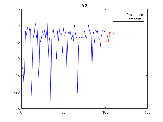
Forecast the LSETAR model into a 50-period horizon. Specify the endogenous threshold variable and its delay.
fh = 50;
YF = forecast(Mdl,Y0F,fh,Index=2,Delay=4);
Y is a 20-by-2 matrix of 20 stepwise forecasted responses from Mdl.
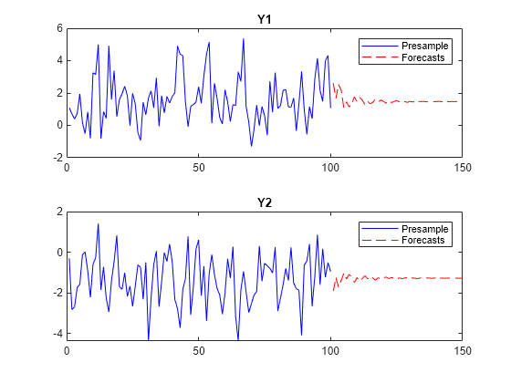
Plot the simulated path and forecasts for each variable on separate plots.
tiledlayout(2,1)
nexttile
plot(1:100,Y0F(:,1),"b",101:(100+fh),YF(:,1),"r--")
title("Y1")
legend(["Presample" "Forecasts"])
nexttile
plot(1:100,Y0F(:,2),"b",101:(100+fh),YF(:,2),"r--")
legend(["Presample" "Forecasts"])
title("Y2")
Consider including regression components for exogenous variables in each submodel of the threshold-switching dynamic regression model in Forecast Multivariate LSETAR Model.
Fully Specify LSETAR Model
Create logistic threshold transitions at mid-levels -1 and 1, with rates 3.5 and 1.5, respectively. Label the states.
t = [-1 1];
r = [3.5 1.5];
stateNames = ["Low" "Med" "High"];
tt = threshold(t,Type="logistic",Rates=[3.5 1.5],StateNames=stateNames)
tt =
  threshold with properties:

          Type: 'logistic'
        Levels: [-1 1]
         Rates: [3.5000 1.5000]
    StateNames: ["Low"    "Med"    "High"]
     NumStates: 3
Assume the following VARX models describe the response processes of the system:
State 1: where
State 2: where
State 3: where
represents a single exogenous variable, represents two exogenous variables, and represents three exogenous variables. Store the submodels in a vector.
% Constants (numSeries x 1 vectors)
C1 = [1; -1];
C2 = [2; -2];
C3 = [3; -3];

% Regression coefficients (numSeries x numRegressors matrices)
Beta1 = [1; -1];            % 1 regressor
Beta2 = [2 2; -2 -2];       % 2 regressors
Beta3 = [3 3 3; -3 -3 -3];  % 3 regressors

% Autoregression coefficients (numSeries x numSeries matrices)
AR1 = {};
AR2 = {[0.5 0.1; 0.5 0.5]};
AR3 = {[0.25 0; 0 0] [0 0; 0.25 0]};

% Innovations covariances (numSeries x numSeries matrices)
Sigma1 = [1 -0.1; -0.1 1];
Sigma2 = [2 -0.2; -0.2 2];
Sigma3 = [3 -0.3; -0.3 3];

% VARX submodels
mdl1 = varm(Constant=C1,AR=AR1,Beta=Beta1,Covariance=Sigma1);
mdl2 = varm(Constant=C2,AR=AR2,Beta=Beta2,Covariance=Sigma2);
mdl3 = varm(Constant=C3,AR=AR3,Beta=Beta3,Covariance=Sigma3);

mdl = [mdl1; mdl2; mdl3];
Create an LSETAR model from the switching mechanism tt and the state-specific submodels mdl. Label the series Y1 and Y2.
Mdl = tsVAR(tt,mdl,SeriesNames=["Y1" "Y2"]);
Forecast Responses Ignoring Regression Component
If you do not supply exogenous data, forecast ignores the regression components in the submodels.
Obtain a presample, from which to forecast, by simulating one 2-D path of 100 observations from the model. Specify the endogenous threshold variable and its delay, .
rng(1)  % For reproducibility
numObs = 100;
Y0F = simulate(Mdl,numObs,Delay=4,Index=2);
Forecast the LSETAR model into a 50-period horizon. Specify the endogenous threshold variable and its delay.
fh = 50;
YF = forecast(Mdl,Y0F,fh,Index=2,Delay=4);
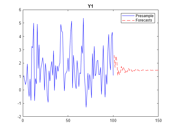
Plot the simulated path and forecasts for each variable on separate plots.
figure;
plot(1:numObs,Y0F(:,1),"b",(numObs+1):(numObs+fh),YF(:,1),"r--")
title("Y1")
legend(["Presample" "Forecasts"])
nexttile
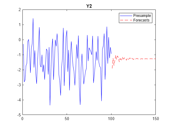
plot(1:numObs,Y0F(:,2),"b",(numObs+1):(numObs+fh),YF(:,2),"r--")
legend(["Presample" "Forecasts"])
title("Y2")
Simulate Data Including Regression Component
To generate random paths from the model, forecast requires expgenous data.
Assume the following AR models for the regressors:
, where .
, where .
, where .
MdlX1 = arima(Constant=1,AR={0.1},Variance=1);
MdlX2 = arima(Constant=2,AR={0 0.2},Variance=2);
MdlX3 = arima(Constant=3,AR={0 0 0.3},Variance=3);
Simulate 100 observations from each model to represent in-sample data for the exogenous predictors.
X10F = simulate(MdlX1,numObs);
X20F = simulate(MdlX2,numObs);
X30F = simulate(MdlX3,numObs);
X0F = [X10F X20F X30F];
Forecast 50 observations from each model to represent exogenous data in the forecast horizon. Specify the simulated in-sample data as a presample.
X1F = forecast(MdlX1,numObs,Y0=X10F);
X2F = forecast(MdlX2,numObs,Y0=X20F);
X3F = forecast(MdlX3,numObs,Y0=X30F);
XF = [X1F X2F X3F];
Obtain presample response data, from which to forecast, by simulating one 2-D path of 100 observations from the model. Specify the endogenous threshold variable and its delay, and specify the simulated exogenous data.
Y0FX = simulate(Mdl,numObs,Delay=4,Index=2,X=X0F);
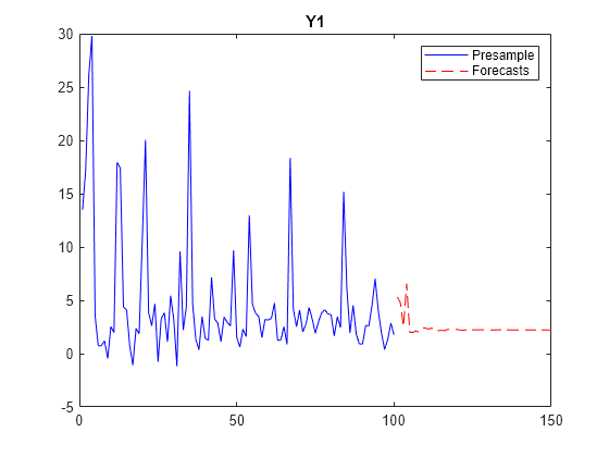
Forecast the LSETAR model into a 50-period horizon. Specify the endogenous threshold variable and its delay, and specify the exogenous data in the forecast horizon.
YFX = forecast(Mdl,Y0FX,fh,Index=2,Delay=4,X=XF);

figure;
plot(1:numObs,Y0FX(:,1),"b",(numObs+1):(numObs+fh),YFX(:,1),"r--")
title("Y1")
legend(["Presample" "Forecasts"])
nexttile
plot(1:numObs,Y0FX(:,2),"b",(numObs+1):(numObs+fh),YFX(:,2),"r--")
legend(["Presample" "Forecasts"])
title("Y2")
Input Arguments
Name-Value Arguments
Output Arguments
Tips
References
Version History
Introduced in R2021b