Backtest Investment Strategies Using datetime and calendarDuration
This example shows how to use datetime inputs in the backtesting workflow. Backtesting is a useful tool to compare how investment strategies perform over historical or simulated market data. Using datetime inputs allows you to accurately specify the exact days that you can then use during the investment period to obtain initial weights from a warm up period, to select a start date to begin the backtest, and to establish a rebalancing frequency.
Load Data
The backtesting framework requires adjusted asset prices, meaning prices adjusted for dividends, splits, or other events. The prices must be stored in a MATLAB® timetable with each column holding a time series of asset prices for an investable asset.
In this example, you use the closing prices of the Dow Jones Industrial Average for 2006.
% Read a table of daily adjusted close prices for 2006 DJIA stocks.
T = readtable('dowPortfolio.xlsx');

% For readability, use only 15 of the 30 DJI component stocks.
assetSymbols = ["AA","CAT","DIS","GM","HPQ","JNJ","MCD","MMM","MO","MRK","MSFT","PFE","PG","T","XOM"];

% Prune the table to hold only the dates and selected stocks.
timeColumn = "Dates";
T = T(:,[timeColumn assetSymbols]);

% Convert to the table to a timetable.
pricesTT = table2timetable(T,'RowTimes','Dates');

% View the structure of the prices timetable.
head(pricesTT)
       Dates        AA       CAT      DIS      GM       HPQ      JNJ      MCD      MMM      MO       MRK     MSFT      PFE      PG        T       XOM
    ___________    _____    _____    _____    _____    _____    _____    _____    _____    _____    _____    _____    _____    _____    _____    _____

    03-Jan-2006    28.72    55.86    24.18    17.82    28.35    59.08    32.72    75.93    52.27    30.73    26.19    22.16    56.38     22.7    56.64
    04-Jan-2006    28.89    57.29    23.77     18.3    29.18    59.99    33.01    75.54    52.65    31.08    26.32    22.88    56.48    22.87    56.74
    05-Jan-2006    29.12    57.29    24.19    19.34    28.97    59.74    33.05    74.85    52.52    31.13    26.34     22.9     56.3    22.92    56.45
    06-Jan-2006    29.02    58.43    24.52    19.61     29.8    60.01    33.25    75.47    52.95    31.08    26.26    23.16    56.24    23.21    57.57
    09-Jan-2006    29.37    59.49    24.78    21.12    30.17    60.38    33.88    75.84    53.11    31.58    26.21    23.16    56.67     23.3    57.54
    10-Jan-2006    28.44    59.25    25.09    20.79    30.33    60.49    33.91    75.37    53.04    31.27    26.35    22.77    56.45    23.16    57.99
    11-Jan-2006    28.05    59.28    25.33    20.61    30.88    59.91     34.5    75.22    53.31    31.39    26.63    23.06    56.65    23.34    58.38
    12-Jan-2006    27.68    60.13    25.41    19.76    30.57    59.63    33.96    74.57    53.23    31.41    26.48     22.9    56.02    23.24    57.77
Define the Strategies
You use backtestStrategy to define investment strategies that capture the logic used to make asset allocation decisions while a backtest is running. Each strategy is periodically given the opportunity to update its portfolio allocation. When you use backtestStrategy, you specify the allocation frequency with the RebalanceFrequency name-value argument. This argument can be an integer, a duration object, a calendarDuration object, or a datetime object.
This example uses two backtesting strategies:
Equal-weighted portfolio
Maximum Sharpe ratio portfolio
, where an vector of returns and is the covariance matrix.
Compute Initial Weights
By default, the initial weights allocate all capital to cash. To avoid this, the first two months (January and February) of the data are used to estimate the initial weights for the different strategies.
t0 = datetime(2006,1,1);
tEnd = datetime(2006,2,28);
warmupPeriod = t0:tEnd;
You calculate the initial weights by calling the backtestStrategy rebalance functions with only the dates in January and February.
% No current weights (100% cash position).
numAssets = size(pricesTT,2);
current_weights = zeros(1,numAssets);

% Warm-up partition of data set timetable.
warmupTT = pricesTT(warmupPeriod,:);

% Compute the initial portfolio weights for each strategy.
equalWeight_initial     = equalWeightFcn(current_weights,warmupTT);
maxSharpeRatio_initial  = maxSharpeRatioFcn(current_weights,warmupTT);
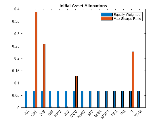
Visualize the initial weight allocations from the strategies.
strategyNames = {'Equally Weighted', 'Max Sharpe Ratio'};
assetSymbols = pricesTT.Properties.VariableNames;
initialWeights = [equalWeight_initial(:), maxSharpeRatio_initial(:)];
bar(assetSymbols,initialWeights);
legend(strategyNames);
title('Initial Asset Allocations');
Create Backtest Strategies
In this example the rebalancing frequency of the strategies is set to the first available day of each month.
% Rebalance at the beginning of the month.
tEnd = datetime(2006,12,31);
rebalFreq = t0:calmonths(1):tEnd;
The lookback window defines the minimum and maximum amount of data to consider when rebalancing. In this example, the rebalance occurs if the backtest start time is at least 2 months prior to the rebalancing time, and it will not include prices older than 6 calendar months.
% Set the rolling lookback window to be at least 2 calendar months and at
% most 6 calendar months.
minLookback = calmonths(2);
maxLookback = calmonths(6);
lookback  = [minLookback maxLookback];

% Use a fixed transaction cost (buy and sell costs are both 0.5% of amount
% traded).
transactionsFixed = 0.005;

% Define backtest strategies
strat1 = backtestStrategy('Equal Weighted', @equalWeightFcn, ...
    'RebalanceFrequency', rebalFreq, ...
    'LookbackWindow', lookback, ...
    'TransactionCosts', transactionsFixed, ...
    'InitialWeights', equalWeight_initial);

strat2 = backtestStrategy('Max Sharpe Ratio', @maxSharpeRatioFcn, ...
    'RebalanceFrequency', rebalFreq, ...
    'LookbackWindow', lookback, ...
    'TransactionCosts', transactionsFixed, ...
    'InitialWeights', maxSharpeRatio_initial);

% Aggregate the strategy objects into an array.
strategies = [strat1, strat2];
Run the Backtest
Set an annual risk-free rate of 1%.
% 1% annual risk-free rate
annualRiskFreeRate = 0.01;
Create the backtestEngine object using the two previously defined strategies. If the rebalancing date is missing in the prices timetable (this usually happens when the day falls on a weekend or a holiday), rebalance on the next available date.
% Create the backtesting engine object
backtester = backtestEngine(strategies,'RiskFreeRate',annualRiskFreeRate,...
    'DateAdjustment','Next');
Use runBacktest to run the backtest. Since this example uses the first two months of data to find the initial weights, use the 'Start' name-value argument to initiate the backtesting after the warm-up period. This is done to avoid the look-ahead bias (that is, "seeing the future").
backtester = runBacktest(backtester,pricesTT,'Start',warmupPeriod(end));Examine Backtest Results
Use the summary function to generate a table of strategy performance results for the backtest.
summaryByStrategies = summary(backtester)
summaryByStrategies=9×2 table
                       Equal_Weighted    Max_Sharpe_Ratio
                       ______________    ________________

    TotalReturn             0.19615           0.097125
    SharpeRatio             0.13059            0.04967
    Volatility            0.0063393          0.0088129
    AverageTurnover      0.00076232           0.012092
    MaxTurnover            0.030952            0.68245
    AverageReturn        0.00086517         0.00047599
    MaxDrawdown            0.072652            0.11764
    AverageBuyCost          0.04131            0.63199
    AverageSellCost         0.04131            0.63199
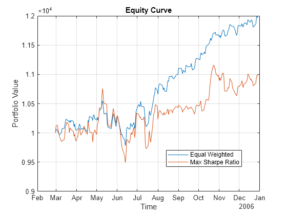
Use equityCurve to plot the equity curve for the different investment strategies.
equityCurve(backtester)

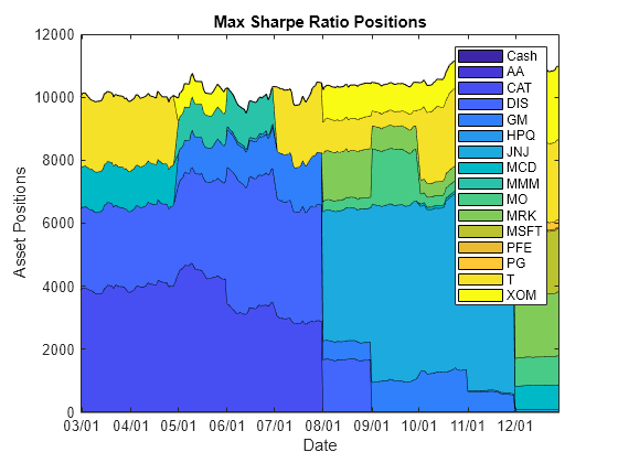
You can visualize the change in the strategy allocations over time using an area chart of the daily asset positions. For information on the assetAreaPlot function, see the Local Functions section.
strategyName = 'Max_Sharpe_Ratio';
assetAreaPlot(backtester,strategyName)
Local Functions
function new_weights = equalWeightFcn(~,pricesTT)
% Equal-weighted portfolio allocation

nAssets = size(pricesTT, 2);
new_weights = ones(1,nAssets);
new_weights = new_weights / sum(new_weights);

end
function new_weights = maxSharpeRatioFcn(~,pricesTT)
% Max Sharpe ratio portfolio allocation

nAssets = size(pricesTT, 2);
assetReturns = tick2ret(pricesTT);
% Max 25% into a single asset (including cash)
p = Portfolio('NumAssets',nAssets,...
    'LowerBound',0,'Budget',1);
p = estimateAssetMoments(p,assetReturns{:,:});
new_weights = estimateMaxSharpeRatio(p);

end
function assetAreaPlot(backtester,strategyName)
% Plot the asset allocation as an area plot.

t = backtester.Positions.(strategyName).Time;
positions = backtester.Positions.(strategyName).Variables;
h = area(t,positions);
title(sprintf('%s Positions',strrep(strategyName,'_',' ')));
xlabel('Date');
ylabel('Asset Positions');
xtickformat('MM/dd');
xlim([t(1) t(end)])
oldylim = ylim;
ylim([0 oldylim(2)]);
cm = parula(numel(h));
for i = 1:numel(h)
    set(h(i),'FaceColor',cm(i,:));
end
legend(backtester.Positions.(strategyName).Properties.VariableNames)

end