Hydromechanical 3-Way Directional Valve with Position Input
R2026bThis example shows how to build a 3-way directional valve using components from the Hydromechanical Valves library and compares it to the behavioral 3-Way Directional Valve (IL) block.
model = "Hydromechanical3WayDirectionalValve";
open_system(model)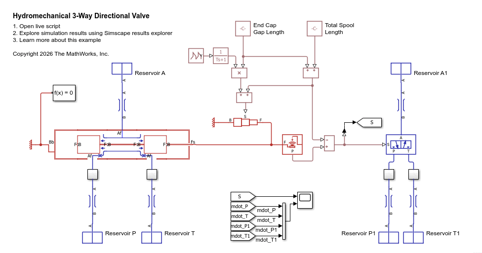
Model Overview
Each block in the Hydromechanical Valves library models a piece of a valve that you combine to model a complete valve. The block icons are intended to be arranged next to each other to resemble a valve schematic, but they must still be connected together via their B and F hydromechanical valve ports. The following picture shows the model with the individual blocks identified and spaced apart to show the connection lines.
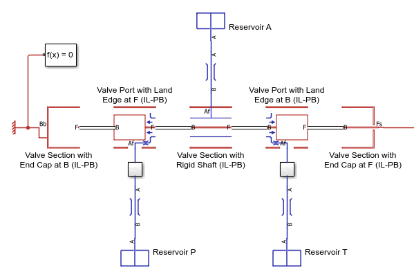
The 3-way directional valve model consists of the following hydromechanical valve blocks:
Valve Section with End Cap at B (IL-PB) - models the terminal section on the left side of the valve and defines the reference position for the entire valve structure.
Valve Port with Land Edge at F (IL-PB) - models the valve port for the first of the two flow paths through the valve along with the left spool land inside the valve body that meters flow through the valve port.
Valve Section with Rigid Shaft (IL-PB) - models the section between the two valve ports and the spool shaft inside the valve body that rigidly connects the two lands.
Valve Port with Land Edge at B (IL-PB) - models the valve port for the second of the two flow paths through the valve along with the right spool land inside the valve body that meters flow through the valve port.
Valve Section with End Cap at F (IL-PB) - models the terminal section on the right side of the valve and provides a connection point for the valve actuator that moves the spool.
For more information, see Get Started with the Hydromechanical Valve Library.
Model Setup
The model Hydromechanical3WayDirectionalValve is already fully configured and ready to simulate a 3-way directional valve. This section highlights the key steps in configuring the model.
Fluid enters the valve structure via port Af in Valve Port with Rigid Shaft (IL-PB). This port provides a direct isothermal liquid network connection to the fluid inside the valve. To model this connection, configure the valve section to contain liquid and to expose the isothermal liquid port Af:
set_param(model + "/Valve Section with Rigid Shaft (IL-PB)", "contains_liquid", "true")
set_param(model + "/Valve Section with Rigid Shaft (IL-PB)", "enable_liquid_port", "true")
Once the fluid is inside the valve, it flows toward either the left valve port or the right valve port. Depending on the position of the spool relative to the valve body, the left valve port will be uncovered by the left spool land and the right valve port will be covered by the right spool land or vice versa. This movement lets the fluid flow out one of the two valve ports.
The two spool lands block fluid flow inside the valve. Therefore, the two end cap valve sections on the other side of the two spool lands do not contain fluid. When a valve section is configured to contain no fluid, the block assumes it is open to the atmosphere.
set_param(model + "/Valve Section with End Cap at B (IL-PB)", "contains_liquid", "false")
set_param(model + "/Valve Section with End Cap at F (IL-PB)", "contains_liquid", "false")
Note that if you do not set contains_liquid to false in the two end cap valve sections, the icons will show the blue isothermal liquid lines to indicate that there is fluid inside. The blue lines will not match up with any blue lines in the adjacent valve port block icons. This mismatch in adjacent icons is a visual indication that the model is not configured correctly.
All mechanical models, including hydromechanical valve models, need a reference point to define the zero position. In this model, the left end cap is the reference position. Therefore, expose the position-based translational port Bb for the valve body and connect it to the Translational World (PB) block.
set_param(model + "/Valve Section with End Cap at B (IL-PB)", "enable_cap_port", "true")
In order to move the spool, you need a connection point to connect an actuator. Expose a position-based translational port Fs for the spool on the right end cap and connect it to a Length Actuator (PB) block.
set_param(model + "/Valve Section with End Cap at B (IL-PB)", "enable_shaft_port", "true")
Model Parameters
After configuring the model, parameterize the blocks to define the spacing between the valve ports along the valve body and between the lands along the spool. When referring to the geometry, the "valve axial direction" refers to the translational motion direction of the moving valve element, which is the spool in this model. The "radial direction" and the "circumferential direction" are then defined assuming that the valve is axisymmetric.
Model the two valve ports as simple rectangular slots with the same width along the valve axis and length along the circumference:
W_port = 0.01; % m
L_port = 0.01; % m
set_param(model + "/Valve Port with Land Edge at F (IL-PB)", "port_width", "W_port")
set_param(model + "/Valve Port with Land Edge at F (IL-PB)", "port_length", "L_port")
set_param(model + "/Valve Port with Land Edge at B (IL-PB)", "port_width", "W_port")
set_param(model + "/Valve Port with Land Edge at B (IL-PB)", "port_length", "L_port")
The spool land width along the valve axis is
W_land = 0.05; % m
set_param(model + "/Valve Port with Land Edge at F (IL-PB)", "land_width", "W_land")
set_param(model + "/Valve Port with Land Edge at B (IL-PB)", "land_width", "W_land")
The fluid inside the valve occupies the annular area around the spool. Therefore, the annular area of the land will experience pressure force from the liquid.
D_land_outer = 0.1; % m
D_land_inner = 0.05; % m
A_land = pi*(D_land_outer^2 - D_land_inner^2)/4
A_land =
0.0059
set_param(model + "/Valve Port with Land Edge at F (IL-PB)", "land_area", "pi*(D_land_outer^2 - D_land_inner^2)/4")
set_param(model + "/Valve Port with Land Edge at B (IL-PB)", "land_area", "pi*(D_land_outer^2 - D_land_inner^2)/4")
The three valve section blocks define the spacing along the valve body to the center of the valve ports. Assume three equal section lengths:
L_body = 0.1; % m
set_param(model + "/Valve Section with End Cap at B (IL-PB)", "body_length", "L_body")
set_param(model + "/Valve Section with Rigid Shaft (IL-PB)", "body_length", "L_body")
set_param(model + "/Valve Section with End Cap at F (IL-PB)", "body_length", "L_body")
The middle valve section block also define the spacing between the two spool lands:
L_shaft = 0.06; % m
set_param(model + "/Valve Section with Rigid Shaft (IL-PB)", "shaft_length", "L_shaft")
An extra shaft is connected to the right spool land and extends out beyond the right end cap. The actuator is attached to the end of this extra shaft.
L_shaft_end = 0.2; % m
set_param(model + "/Valve Section with End Cap at F (IL-PB)", "shaft_length", "L_shaft_end")
Finally, specify the area of the fluid channels connected to the valve ports, which refers to the fluid channels beyond the valve bore, such as the fluid passages machined into the larger valve housing or the external pipes connected to the outer valve ports. While the hydromechanical valve blocks do not model these fluid channels themselves, the purpose of this parameter is to provide some pressure loss even when the valve port is fully uncovered based on the area ratio of the valve port to the connecting fluid channels.
A_conn = 2e-4; % m^2
set_param(model + "/Valve Port with Land Edge at F (IL-PB)", "connecting_area", "A_conn")
set_param(model + "/Valve Port with Land Edge at B (IL-PB)", "connecting_area", "A_conn")
Simulate with Position Input
In this example, you motion actuate the valve by specifying the position of the end of the spool shaft as a function of time. First, determine the maximum amount that the spool can move.
The total valve body length is
L_body_total = 3*L_body
L_body_total =
0.3000
and the total internal spool length is
L_spool_internal = 2*W_land + L_shaft
L_spool_internal =
0.1600
These values let us calculate the gap length between the end cap and the spool when the spool is at the neutral center position. Let the actuator move the spool by up to this gap length in the positive and negative direction.
L_gap = (L_body_total - L_spool_internal)/2
L_gap =
0.0700
set_param(model + "/End Cap Gap Length", "constant", "(3*L_body - 2*W_land - L_shaft)/2")
The total spool length including the extra shaft at the end cap is
L_spool_total = L_spool_internal + L_shaft_end
L_spool_total =
0.3600
set_param(model + "/Total Spool Length", "constant", "2*W_land + L_shaft + L_shaft_end")
Therefore, the neutral center position for the actuator is
L_act_neutral = L_gap + L_spool_total
L_act_neutral =
0.4300
Actuate the valve by first moving the spool in the positive direction, then in the negative direction, then back to then neutral position. When the spool is moved in the positive direction, the left spool land will cover the left valve port and the right spool land will uncover the right valve port. Therefore, the fluid flow path will be between Reservoir A and Reservoir T. When the spool is moved in the negative direction, the left spool land will uncover the left valve port and the right spool land will cover the right valve port. Therefore, the fluid flow path will be between Reservoir A and Reservoir P.
Because the motion of the spool is prescribed, you do not need to provide an initial condition for the spool position.
Simulate the model and observe the results in the scope. The mass flow rate mdot_P is the fluid flow through the left valve port to Reservoir P. The mass flow rate mdot_T is the fluid flow through the right valve port to Reservoir T. The two mass flow rates are different because the pressures in Reservoir P and Reservoir T are different.
open_system(model + "/Scope")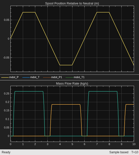
sim(model)
Using the logged data, you can plot the opening distance and the metering area for the two valve port and spool land combinations. The opening distance is the distance between the land edge and the valve port edge. The block defines the value of zero to be when the two edges are on top of each other. The metering area is the area between the land edge and the valve port edge that restricts fluid flow. As the opening distance increases, the metering area increases to permit more flow.
First, extract the desired simulation results from the logged data:
t = simlog_Hydromechanical3WayDirectionalValve.Valve_Port_with_Land_Edge_at_F_IL_PB.opening.series.time;
opening_left  = simlog_Hydromechanical3WayDirectionalValve.Valve_Port_with_Land_Edge_at_F_IL_PB.opening.series.values("m");
opening_right = simlog_Hydromechanical3WayDirectionalValve.Valve_Port_with_Land_Edge_at_B_IL_PB.opening.series.values("m");
area_left  = simlog_Hydromechanical3WayDirectionalValve.Valve_Port_with_Land_Edge_at_F_IL_PB.metering_area.series.values("m^2");
area_right = simlog_Hydromechanical3WayDirectionalValve.Valve_Port_with_Land_Edge_at_B_IL_PB.metering_area.series.values("m^2");
Next, generate the plot:
figure
tiledlayout(2, 1)
ax(1) = nexttile;
plot(t, opening_left, t, opening_right, LineWidth = 1)
grid on
title("Opening Distance")
ylabel("Opening Distance (m)")
legend("Left Valve Port", "Right Valve Port", Location = "southoutside", Orientation = "horizontal")
ax(2) = nexttile;
plot(t, area_left, t, area_right, LineWidth = 1)
grid on
title("Metering Area")
ylabel("Metering Area (m^2)")
xlabel("Time (s)")
linkaxes(ax, "x")
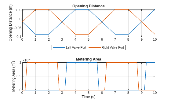
The opening distances for the left valve port and right valve port are mirror images of each other because when one valve port opens, the other one closes. The metering area remains closed until the opening distance rises above 0 m. The metering area then increases until it reaches the valve port area, after which further increases in opening distance no longer increases the metering area. The valve port area is
A_port = W_port * L_port
A_port =
1.0000e-04
Because the spool land width is greater than the valve port width, this 3-way directional valve is overlapped. Whenever the spool is near the neutral center position, both opening distances negative and thus both metering areas are closed, blocking both fluid flow paths.
Comparison to Behavioral Valve
The Hydromechanical Valves library lets you build up complex customized valves based on the geometry of the valve structure. Other blocks in the Valves & Orifices library are behavioral components because they model the behavior of the valve without considering the detailed geometry and mechanical effects of the valve structure. For common valve configurations, the more detailed hydromechanical valve model and the simpler behavioral valve model can produce the same results. This example compares the hydromechanical 3-way directional valve to the behavioral 3-Way Directional Valve (IL) block and shows how the geometrical parameters of the hydromechanical valve map to the behavioral valve.
In the behavioral valve, the spool travel refers only to the distance from when the valve port is closed to when the valve port is open, even if the spool can actually travel a greater distance. Therefore, it is just the valve port width:
set_param(model + "/3-Way Directional Valve (IL)", "del_S_max", "W_port")
The maximum orifice area is the valve port area and the minimum orifice area is by default in the hydromechanical valve a factor of 1e-6 smaller:
set_param(model + "/3-Way Directional Valve (IL)", "area_max", "W_port * L_port")
set_param(model + "/3-Way Directional Valve (IL)", "area_leak", "W_port * L_port * 1e-6")
The cross-sectional area at ports A, P, and T of the behavioral valve is equivalent to the area of the fluid channels connected to the valve ports:
set_param(model + "/3-Way Directional Valve (IL)", "area", "A_conn")
Lastly, determine the spool position relative to the neutral position at which the orifice area (i.e., the metering area) is at the maximum. From the center of the valve, the center of the valve port is located at a distance L_body/2 away and so the far edge of the valve port is located at a distance L_body/2 + W_port/2 away. Also from the center of the valve, the spool land edge is located at a distance L_shaft/2 away. The metering area is maximum when the spool land edge is at the same location as the far valve port edge. This distance is therefore
S_max = (L_body + W_port - L_shaft)/2
S_max =
0.0250
set_param(model + "/3-Way Directional Valve (IL)", "S_max_PA", "-(L_body + W_port - L_shaft)/2")
set_param(model + "/3-Way Directional Valve (IL)", "S_max_AT", "(L_body + W_port - L_shaft)/2")
Simulate the model and observe the results in the scope. The mass flow rates mdot_P1 and mdot_T1 are the same as mdot_P and mdot_T but for the behavioral valve instead of the hydromechanical valve. The results show the same mass flow rates for the behavioral valve and the hydromechanical valve using the parameter mapping above.
open_system(model + "/Scope")
sim(model)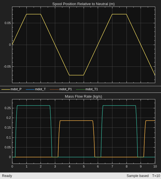
You can also use the logged data to compare the metering areas. First, extract the simulation results for the hydromechanical valve and the behavioral valve. The left valve port and land corresponds to orifice PA in the behavioral valve, and the right valve port and land corresponds to orifice AT in the behavioral valve.
t = simlog_Hydromechanical3WayDirectionalValve.Valve_Port_with_Land_Edge_at_F_IL_PB.metering_area.series.time;
area_left  = simlog_Hydromechanical3WayDirectionalValve.Valve_Port_with_Land_Edge_at_F_IL_PB.metering_area.series.values("m^2");
area_right = simlog_Hydromechanical3WayDirectionalValve.Valve_Port_with_Land_Edge_at_B_IL_PB.metering_area.series.values("m^2");
mdot_left  = -simlog_Hydromechanical3WayDirectionalValve.Valve_Port_with_Land_Edge_at_F_IL_PB.mdot_Af.series.values("kg/s");
mdot_right = -simlog_Hydromechanical3WayDirectionalValve.Valve_Port_with_Land_Edge_at_B_IL_PB.mdot_Af.series.values("kg/s");

area_left_behavioral  = simlog_Hydromechanical3WayDirectionalValve.x3_Way_Directional_Valve_IL.orifice_PA.orifice_area.series.values("m^2");
area_right_behavioral = simlog_Hydromechanical3WayDirectionalValve.x3_Way_Directional_Valve_IL.orifice_AT.orifice_area.series.values("m^2");
mdot_left_behavioral  = simlog_Hydromechanical3WayDirectionalValve.x3_Way_Directional_Valve_IL.orifice_PA.mdot_B.series.values("kg/s");
mdot_right_behavioral = simlog_Hydromechanical3WayDirectionalValve.x3_Way_Directional_Valve_IL.orifice_AT.mdot_A.series.values("kg/s");
Next, generate the plot:
figure
tiledlayout(2, 1)
ax(1) = nexttile;
plot(t, area_left, "-", t, area_right, "-", LineWidth = 1)
hold on
plot(t, area_left_behavioral, "--", t, area_right_behavioral, "--", LineWidth = 1)
hold off
grid on
title("Metering Area")
ylabel("Metering Area (m^2)")
legend("Left Port", "Right Port", "Left Port Behavioral", "Right Port Behavioral", ...
    Location = "southoutside", Orientation = "horizontal")
ax(2) = nexttile;
plot(t, mdot_left, "-", t, mdot_right, "-", LineWidth = 1)
hold on
plot(t, mdot_left_behavioral, "--", t, mdot_right_behavioral, "--", LineWidth = 1)
hold off
grid on
title("Mass Flow Rate")
ylabel("Mass Flow Rate (kg/s)")
xlabel("Time (s)")
linkaxes(ax, "x")
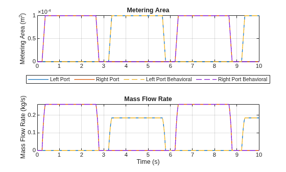
The metering areas and the mass flow rates match between the hydromechanical valve and the behavioral valve.
Model Valve Forces
One use case for the Hydromechanical Valves library is to model the forces on the valve structure and simulate the dynamic response of the moving spool or poppet. The blocks model fluid pressure forces on the spool land and piston surfaces, as indicated by the small blue arrows in the block icons. The blocks use gauge pressure to calculate pressure forces because the sides of the land or piston that do not contain liquid are assumed to be open to the atmosphere.
In addition to pressure forces, you can model flow momentum force due to the changing direction of the fluid jet as it passes through the metering area. Use the von Mises jet angle model to obtain a rough estimate of the flow momentum forces:
set_param(model + "/Valve Port with Land Edge at F (IL-PB)", "flow_force_model", ...
    "fluids.isothermal_liquid.valves_orifices.hydromechanical_valves.enum.SpoolFlowForceModel.VonMisesJetAngle")
set_param(model + "/Valve Port with Land Edge at B (IL-PB)", "flow_force_model", ...
    "fluids.isothermal_liquid.valves_orifices.hydromechanical_valves.enum.SpoolFlowForceModel.VonMisesJetAngle")
When using the von Mises jet angle model, you need to provide the radial clearance between the outer diameter of the spool land and the valve body:
h_clearance = 5e-6; % m
set_param(model + "/Valve Port with Land Edge at F (IL-PB)", "radial_clearance", "h_clearance")
set_param(model + "/Valve Port with Land Edge at B (IL-PB)", "radial_clearance", "h_clearance")
In this example, the fluid forces, or any other forces, do not matter because the spool position is prescribed. Therefore, there is no dynamic response and spool mass has no effect. In fact, if you enable land mass in the model, it is best practice to drive the spool position with a second-order continuous (i.e., smooth) signal so that the spool acceleration is well-defined.
Although a position-driven valve model does not have a dynamic response, it can still be useful to simulate and observe the forces that the valve actuator would encounter during the simulation to estimate the required size of the actuator.
close_system(model + "/Scope")
sim(model)
Extract the pressure forces and flow momentum forces on the left and right spool land from the logged data:
t = simlog_Hydromechanical3WayDirectionalValve.Valve_Port_with_Land_Edge_at_F_IL_PB.f_pressure.series.time;
pressure_force_left  = simlog_Hydromechanical3WayDirectionalValve.Valve_Port_with_Land_Edge_at_F_IL_PB.f_pressure.series.values("N");
pressure_force_right = simlog_Hydromechanical3WayDirectionalValve.Valve_Port_with_Land_Edge_at_B_IL_PB.f_pressure.series.values("N");
flow_force_left  = simlog_Hydromechanical3WayDirectionalValve.Valve_Port_with_Land_Edge_at_F_IL_PB.f_flow.series.values("N");
flow_force_right = simlog_Hydromechanical3WayDirectionalValve.Valve_Port_with_Land_Edge_at_B_IL_PB.f_flow.series.values("N");
Next, generate the plot:
figure
tiledlayout(2, 1)
ax(1) = nexttile;
plot(t, pressure_force_left, t, pressure_force_right, LineWidth = 1)
grid on
title("Pressure Force")
ylabel("Force (N)")
legend("Left Valve Port", "Right Valve Port", Location = "southoutside", Orientation = "horizontal")
ax(2) = nexttile;
plot(t, flow_force_left, t, flow_force_right, LineWidth = 1)
grid on
title("Flow Momentum Force")
ylabel("Force (N)")
xlabel("Time (s)")
linkaxes(ax, "x")
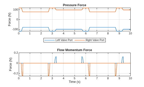
In this model, the pressure forces cancel out each other because the fluid is simply sandwiched between the two spool lands. The flow momentum forces do not cancel. They are concentrated around when the valve just starts to open and when the valve is almost closed. However, the magnitude of the flow momentum forces in this model are very small.

