Visualize Density Using Geographic Density Plots

This example shows how to visualize the relative distribution of points in latitude and longitude coordinates by using a geographic density plot. Density plots are useful for visualizing large or tightly clustered data sets.

A density plot is a type of heatmap. Other types of heatmaps that you can create on maps include:

• Choropleth maps, which display the values of numeric attributes within polygons. For an example, see Create Choropleth Map from Table Data (Mapping Toolbox).

• Binned scatter plots, which partition points into bins and display the number of points in each bin. For an example, see Create Binned Scatter Plot from Latitude and Longitude Data (Mapping Toolbox).

• Pseudocolor raster plots, which display the values stored in a raster. For examples, see the geopcolor (Mapping Toolbox) reference page.

Load Data

Load a table containing cell tower data for California. Each table row represents a cell tower. The table variables include data about the cell towers, such as the latitude and longitude coordinates and the tower heights. Extract the latitude and longitude coordinates from the table.

load cellularTowers.mat
lat = cellularTowers.Latitude;
lon = cellularTowers.Longitude;

Visualize Using Scatter Plot

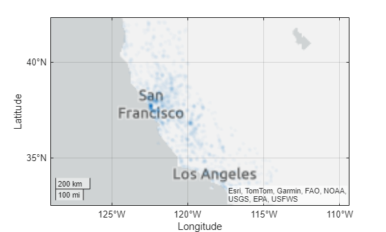
Create a scatter plot from the latitude and longitude coordinates. Note that the scatter plot does not clearly represent the cluster of towers in the region surrounding San Francisco.

geoscatter(lat,lon,".")

Visualize Using Density Plot

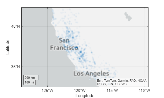
Create a density plot from the coordinates by using the geodensityplot function. By default, the plot visualizes the density of the points by varying the transparency. Regions with high density are more opaque, and regions with low density are more transparent.

figure
geodensityplot(lat,lon)

By default, the density plot uses equal weights for all the data points. Extract the tower heights from the table. Then, create a new density plot that weights the points using the tower heights. The new density plot emphasizes the areas with the tallest towers.

height = cellularTowers.ALLSTRUC;
figure
geodensityplot(lat,lon,height)

By default, the density plot uses the data points to automatically select a radius of influence for each point. Create a new density plot that specifies the radius of influence, in meters, for each point.

radius = 50000;
figure
geodensityplot(lat,lon,height,Radius=radius)

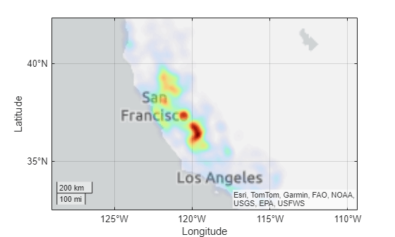
By default, the density plot uses one color. Create a new density plot that uses varying colors by setting the FaceColor name-value argument to "interp". Then, change the colormap. Note that the new density plot visualizes the density of the points using both transparency and color.

figure
geodensityplot(lat,lon,height,Radius=radius,FaceColor="interp")
colormap turbo