Swing-Up Control of Cart-Pole System Using C/GMRES Solver

This example shows how to control a classic underactuated cart-pole system using multistage nonlinear MPC with the C/GMRES solver.

Nonlinear Model of Cart-Pole System

The cart-pole system consists of a cart that can move horizontally and a pendulum (that is, a pole) mounted on the cart, free to swing in the vertical plane. The control input is the horizontal force applied to the cart, $u$. Since the pendulum is not directly actuated, the system is underactuated.

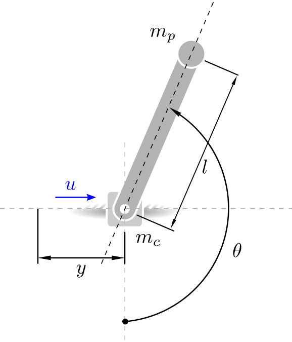
The configuration of the model is determined by the horizon position of the cart, $y$, and the angular position of the pole, $\theta$, resulting in the following state vector:

$x={\left[\begin{array}{cccc}y& \theta & \underset{}{\overset{\dot{}}{y}}& \underset{}{\overset{\dot{}}{\theta }}\end{array}\right]}^T$,

where:

• $y$ is the horizontal position of the cart.

• $\theta$ is the angle of the pole from vertical (zero when pointing down).

• $\underset{}{\overset{\dot{}}{y}}$ is the cart velocity.

• $\underset{}{\overset{\dot{}}{\theta }}$ is the angular velocity of the pole.

The dynamics are nonlinear and are given by the following equations:

$$\begin{array}{l}\underset{}{\overset{¨}{y}}\left(t\right)=\frac{1}{m_c+m_p{\sin }^2\theta \left(t\right)}\left(u+m_p\sin \theta \left(t\right)\left(l{\underset{}{\overset{\dot{}}{\theta }}}^2\left(t\right)+g\cos \theta \left(t\right)\right)\right)\\ \underset{}{\overset{¨}{\theta }}\left(t\right)=\frac{1}{l\left(m_c+m_p{\sin }^2\theta \left(t\right)\right)}\left(-u\cos \theta \left(t\right)-m_{p}l\underset{}{\overset{\dot{}}{\theta }}\left(t\right)\cos \theta \sin \theta -\left(m_c+m_p\right)g\sin \theta \left(t\right)\right)\end{array}$$

The physical parameters of the system are defined in the following table:

Parameter	Value	Units	Description
$$m_c$$	2.0	$$\text{kg}$$	Cart mass
$$m_p$$	0.2	$$\text{kg}$$	Pole mass
$$l$$	0.5	$$m$$	Pole length
$$g$$	9.80665	$$m/s^2$$	Gravitational acceleration

Define a parameter vector containing the physical system parameters:

pvstate = [2; 0.2; 0.5; 9.80665];

Control Objective

The control objective is to swing the pendulum up from the downward position and stabilize it in the upright position while keeping the cart at 1 meter from the origin.

Define initial state.

x0 = zeros(4,1);

Define reference state (upright position at one meter from origin).

xref = [1; pi; 0; 0];

Create a custom chart objects to animate the trajectory obtained with the single-shooting method.

The custom chart object visualizes both the initial and reference state, and is defined in the CartPoleVisualizer.m class file.

figure; 
hPlotSS = CartPoleVisualizer(...
    Y=x0(1),...
    Theta=x0(2),...
    YRef=xref(1),...
    ThetaRef=xref(2),...
    TitleText="Single-Shooting");

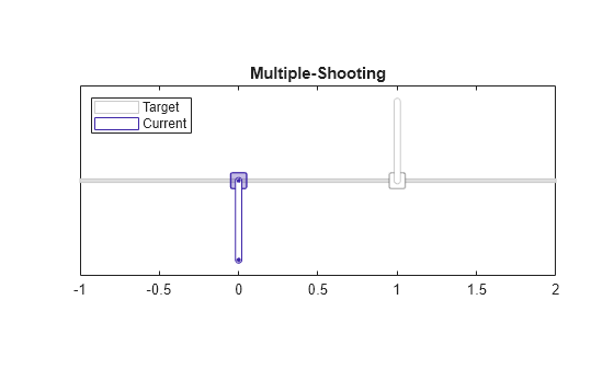
Create a custom chart objects to animate the trajectory obtained with the multiple-shooting method.

figure; 
hPlotMS = CartPoleVisualizer(...
    Y=x0(1),...
    Theta=x0(2),...
    YRef=xref(1),...
    ThetaRef=xref(2),...
    TitleText="Multiple-Shooting");

MPC is optimizes a performance index over a finite time horizon. To achieve the control objective, define a performance index $J$ that penalizes both deviations from the target state and large control inputs.

$$J=\frac{1}{2}{\Vert x\left(T\right)-\underset{}{\overset{‾}{x}}\Vert }_{S_f}^2+{\int }_t^{t+T}\frac{1}{2}\left({\Vert x\left(t\right)-\underset{}{\overset{‾}{x}}\Vert }_Q^2+{\Vert u\left(t\right)\Vert }_R^2\right)\text{dt}$$

Here:

• $\underset{}{\overset{‾}{x}}$ represents the desired state (upright pole and cart at 1 meter from the origin).

• $S_f$, $Q$, and $R$ are weight matrices that determine the importance of different terms in the performance index.

For this example, the weights and objective cost are implemented in the CartPole.m class file, where $S_f=Q=\text{diag}\left(\left[\begin{array}{cccc}2.5& 10& 0.01& 0.01\end{array}\right]\right)$, and $R=1$.

Create Multistage Nonlinear MPC Object

Create a nonlinear multistage MPC object with 100 stages, four states and one input.

p = 100;
msobj = nlmpcMultistage(p,4,1);

Specify the sampling time for the nonlinear multistage MPC object.

msobj.Ts = 0.02;

Specify the prediction model state and Jacobian functions. Use the cart-pole dynamics functions defined in the CartPole.m class file.

% Specify the state transition function
msobj.Model.StateFcn = "CartPole.stateFcn";
msobj.Model.StateJacFcn = "CartPole.stateJacobianFcn";

Specify the running and terminal cost function and their Jacobian. Use the functions defined in the CartPole.m class file. Use the deal function to assign the outputs of the cost and jacobian function to the respective stage properties of msobj.

% Set running cost for the Multistage NLMPC problem
[msobj.Stages(1:p).CostFcn] = deal("CartPole.runningCostFcn");
[msobj.Stages(1:p).CostJacFcn] = deal("CartPole.runningCostJacobianFcn");

% Set terminal cost for the Multistage NLMPC problem
msobj.Stages(p+1).CostFcn = "CartPole.terminalCostFcn";
msobj.Stages(p+1).CostJacFcn = "CartPole.terminalCostJacobianFcn";

Specify number of parameters for both the model and the stage functions.

msobj.Model.ParameterLength = length(pvstate);
[msobj.Stages.ParameterLength] = deal(length(xref));

For more information on specifying cost functions, see Specify Cost Function for Nonlinear MPC.

Set the Optimization Solver

For this example, use the C/GMRES solver. Set the following solver properties:

• MaxIterations = 5

• Restart = 0

Note that by default the C/GMRES solver uses the single-shooting formulation method.

msobj.Optimization.Solver = "cgmres";
msobj.Optimization.SolverOptions.MaxIterations = 5;
msobj.Optimization.SolverOptions.Restart = 0;
disp(msobj.Optimization.SolverOptions)

  Cgmres with properties:

            BarrierParameter: 0.1000
             ConvergenceRate: Inf
                     Display: 'none'
    FiniteDifferenceStepSize: 1.0000e-08
               MaxIterations: 5
         OptimalityTolerance: 1.0000e-06
                     Restart: 0
      StabilizationParameter: 1000
              ShootingMethod: 'single-shooting'
        TerminationTolerance: 1.0000e-06

Generate Code

To speed up computation time during simulation, use getCodeGenerationData and buildMEX.

Generate data structures (coredataSS and onlinedataSS) for the single-shooting method by using getCodeGenerationData.

% Generate constant and run-time data for "single-shooting" method.
msobj.Optimization.SolverOptions.ShootingMethod = "single-shooting";
[coredata_ss, onlinedata_ss] = getCodeGenerationData(msobj,x0,0,...
    StateFcnParameter=pvstate,...
    StageParameter=repmat(xref,p+1,1));

Generate data structures (coredataMS and onlinedataMS) for the multiple-shooting method, again by using getCodeGenerationData.

% Generate constant and run-time data for "multiple-shooting" method.
msobj.Optimization.SolverOptions.ShootingMethod = "multiple-shooting";
[coredata_ms, onlinedata_ms] = getCodeGenerationData(msobj,x0,0,...
    StateFcnParameter=pvstate,...
    StageParameter=repmat(xref,p+1,1));

Generate a MEX function named cartpoleMEXsingleshooting for the single-shooting method. Then generate a second MEX function named cartpoleMEXmultipleshooting for the multiple-shooting method.

if true% Generate MEX functions
    % Generate MEX function for "single-shooting" method.
    msobj.Optimization.SolverOptions.ShootingMethod = "single-shooting";
    buildMEX(msobj, "cartpoleMEXsingleshooting", coredata_ss, onlinedata_ss);

    % Generate MEX function for "multiple-shooting" method.
    msobj.Optimization.SolverOptions.ShootingMethod = "multiple-shooting";
    buildMEX(msobj, "cartpoleMEXmultipleshooting", coredata_ms, onlinedata_ms);
end

Generating MEX function "cartpoleMEXsingleshooting" from your "nlmpcMultistage" object to speed up simulation.
Code generation successful.

MEX function "cartpoleMEXsingleshooting" successfully generated.

Generating MEX function "cartpoleMEXmultipleshooting" from your "nlmpcMultistage" object to speed up simulation.
Code generation successful.

MEX function "cartpoleMEXmultipleshooting" successfully generated.

Simulate Closed Loop (Single-Shooting)

Simulate the closed-loop performance obtained using the single-shooting method. At each step, integrate the cart-pole system dynamics forward in time using the state equations and apply the control input returned by the single-shooting controller.

FinalTime = 20;     % Simulation duration
xss = x0;           % Initialize state
uss = 0;            % Initialize control input
Ts = 1e-3;          % Sampling time for simulation

% Initialize data storage
N = FinalTime/Ts;
xHistorySS = zeros(N+1,4);
uHistorySS = zeros(N+1,1);

% Main simulation loop
for ct = 0:N
    % Compute optimal control move
    [uss,onlinedata_ss] = ...
    cartpoleMEXsingleshooting(xss, uss, onlinedata_ss);

    % Update plant state (Euler update)
    xss = xss + CartPole.stateFcn(xss,uss,pvstate)*Ts;

    % Store results
    xHistorySS(ct+1,:) = xss;
    uHistorySS(ct+1,:) = uss;

    % Update underactuated two-link robot plot.
    hPlotSS.Y = xss(1);
    hPlotSS.Theta = xss(2);
    drawnow limitrate
end

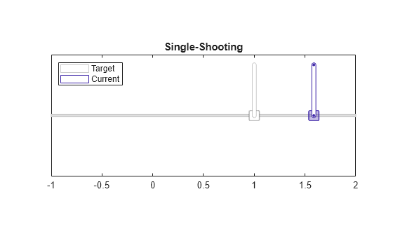
The multistage single-shooting controller swings up and balances the pole upright but overshoots the desired position.

Simulate Closed Loop (Multiple-Shooting)

Simulate the closed-loop performance obtained using the multiple-shooting method. At each step, integrate the cart-pole system dynamics forward in time using the state equations and apply the control input returned by the multiple-shooting controller.

FinalTime = 20;     % Simulation duration
xms = x0;           % Initialize state
ums = 0;            % Initialize control input
Ts = 1e-3;          % Sampling time for simulation

% Initialize data storage
N = FinalTime/Ts;
xHistoryMS = zeros(N+1,4);
uHistoryMS = zeros(N+1,1);

% Main simulation loop
for ct = 0:N
    % Compute optimal control move
    [ums,onlinedata_ms] = cartpoleMEXmultipleshooting(xms, ums, onlinedata_ms);

    % Update plant state (Euler update)
    xms = xms + CartPole.stateFcn(xms,ums,pvstate)*Ts;

    % Store results
    xHistoryMS(ct+1,:) = xms;
    uHistoryMS(ct+1,:) = ums;

    % Update underactuated two-link robot plot.
    hPlotMS.Y = xms(1);
    hPlotMS.Theta = xms(2);
    drawnow limitrate
end

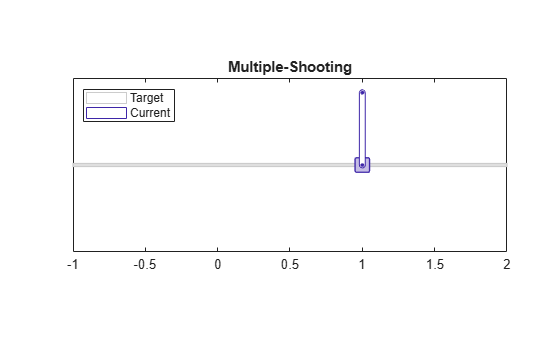
The multistage multiple-shooting controller swings up and balances the pole upright and also drives it to the desired position. This results is mostly due to the generally better numerical robustness of the multiple-shooting algorithm with respect to the single-shooting one.

Plot Results

Plot the states of the cart-pole system over time to visualize the behavior of the system and compare the performance of the single-shooting and multiple-shooting methods. The plots show the cart position, pole angle, cart velocity, and pole angular velocity for both methods, so you can directly compare their effectiveness. Note that the single-shooting method does not reach the 1 meter cart position while the multiple-shooting method achieves it with a steady-state error close to zero.

figure;
tiledlayout(2,2);
ax = gobjects(4,1);
labels = {"y","\theta","\dot{y}","\dot{\theta}"};
for i=1:4
    ax(i) = nexttile();
    hold on;

    plot(0:Ts:FinalTime, xHistorySS(:,i));
    plot(0:Ts:FinalTime, xHistoryMS(:,i));
    plot([0 FinalTime], [xref(i) xref(i)], ':')
    hold off

    % Plot settings
    box on;
    xlabel("Time, $s$",Interpreter="latex")
    ylabel(sprintf("$%s(t)$",labels{i}),Interpreter="latex");
end

% Plot titles
title(ax(1), "Cart Position")
title(ax(2), "Pole Angular Position")
title(ax(3), "Cart Velocity")
title(ax(4), "Pole Angular Velocity")
legend(ax(4), "single-shooting", "multiple-shooting","reference")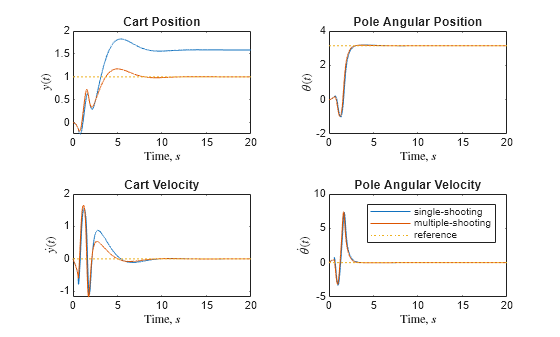

Plot the control input responses for both simulations.

figure;
plot(0:Ts:FinalTime, uHistorySS); hold on;
plot(0:Ts:FinalTime, uHistoryMS); hold off;

% Plot settings
title("Control Input");
ylabel("$u(t)$",Interpreter="latex");
xlabel("Time, $s$",Interpreter="latex");
legend("single-shooting", "multiple-shooting");

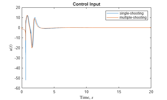
The control input response for single-shooting presents a chattering behavior around 1.2 seconds.

Visualize the trajectory obtained using the multiple-shooting formulation using a CartPoleVisualizer object.

figure;
hPlot = CartPoleVisualizer(...
    Y=xHistoryMS(:,1),...
    Theta=xHistoryMS(:,2), ...
    YRef=xref(1),...
    ThetaRef=xref(2),...
    N=20, ...
    TitleText="Optimal Trajectory");

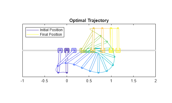
The frames are uniformly spaced in the distance traveled by the tip of the pole, and they transitions from blue to yellow as the simulation progresses through time.