Adaptive Detection for Heterogeneous Clutter and Interference Scenarios

Since R2026a

Introduction

In modern radar systems, adaptive detection faces the critical challenge of identifying target signals in complex environments comprising of thermal noise, interference, and clutter. The fundamental detection problem involves distinguishing between two hypotheses regarding the received signal:

$$\{\begin{array}{ll}{H}_0:y=c,& y_k=c_k,\text{for}k=1,\dots ,K,\\ H_1:y=\alpha s+c,& y_k=c_k,\text{for}k=1,\dots ,K,\end{array}$$

where:

• $$y$$ is the cell under test (CUT) data vector;

• $$c$$ is the colored noise with unknown covariance on the CUT;

• $$y_k$$ is the training data on the k-th training cell;

• $$c_k$$ is the colored noise on the k-th training cell;

• $$s$$ is the steering vector for the signal;

• $$\alpha$$ is the unknown signal complex amplitude.

Space-time adaptive processing (STAP) offers substantial advantages over conventional approaches by simultaneously processing signals in both spatial (antenna array or beam) and temporal (pulse or Doppler) domains. This enables superior separation of targets from interference and clutter as opposed to FFT-based angle-Doppler processing. A conventional STAP radar detection system involves:

• $$N_{rx}$$ received antennas forming the spatial dimension;

• $$N_{pulse}$$ pulses forming the temporal dimension;

• a range-domain CUT data $$y$$ of dimension $$N=N_{tx}{N}_{pulse}$$ that contains potential targets;

• $$K$$ range-domain training cell data $$y_k$$ for noise covariance estimation.

The key challenge lies in developing detectors that maintain constant false alarm rate (CFAR) properties while adapting to unknown noise covariance matrices estimated from limited training data. This requires careful selection of training data and the development of robust covariance estimation techniques that work effectively in practical scenarios with heterogeneous noise environments. Modern approaches to this problem must address computational efficiency, training data requirements, and robustness to non-ideal conditions while maintaining detection performance in increasingly complex electromagnetic environments.

System Setup

Loading the monostatic airborne radar system and generating received data using the setup from the example Introduction to Space-Time Adaptive Processing. The monostatic airborne radar system operates at 10 GHz, transmits 10 coherent pulses and receives the signal over a 6-element uniform linear array (ULA). The radar platform flies at 1,000 meters altitude, moving at a speed that shifts it half an array element spacing per pulse repetition interval (PRI). The received data contains a target along with clutter and a barrage interference. Due to platform motion, ground clutter—modeled using the constant-gamma model (gamma value of −15 dB for wooded terrain)—exhibits angle-dependent Doppler spread. Meanwhile, the interference, located at 60° azimuth and 0° elevation, emits wideband noise that spans the entire Doppler spectrum.

load BasicMonostaticRadarExampleData.mat;
fc = radiator.OperatingFrequency;
c = radiator.PropagationSpeed;
lambda = c/fc;
prf = waveform.PRF;
Fs = waveform.SampleRate;
[receivePulse,tgtpos,tgtmotion,sensorpos,sensormotion,ula,numSamples,numEles,numPulses,intang] = ...
    helperGenerateRadarReceivedData(waveform, radiator, transmitter, collector, receiver);

The ideal target location parameters, including range, azimuth, elevation and Doppler, are given below.

% Target range and angle
tgtLocation = global2localcoord(tgtpos,'rs',sensorpos);
tgtAzimuthAngle = tgtLocation(1);
tgtElevationAngle = tgtLocation(2);
tgtRange = tgtLocation(3);

% Target Doppler
sp = radialspeed(tgtpos, tgtmotion.Velocity, ...
                sensorpos, sensormotion.Velocity);
tgtDp = 2*speed2dop(sp,lambda);
tgtDpNormalized = tgtDp/prf;

% Target range cell index
tgtCellIndex = val2ind(tgtRange, c/(2*Fs));

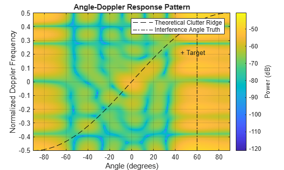
At the target range cell, we analyze the angle-Doppler response by plotting the 2D Fourier transform of the cell-under-test (CUT) data. The target's truth location is marked at approximately 45° azimuth and 0.21 normalized Doppler frequency. For reference, we overlay the predicted clutter ridge characteristic of monostatic radar geometry. The response reveals dominant noise components: the barrage interference appears as a strong vertical line at its azimuth angle, while ground clutter forms the distinctive diagonal ridge. These noise signals completely obscure the target return due to their overwhelming power. This occurs because conventional Fourier processing alone cannot suppress either the spatially localized interference or the Doppler-spread clutter. The result demonstrates why basic spectral analysis fails in this environment and underscores the need for advanced space-time processing to separate the target from noise.

% Angle-Doppler response
tgtData = shiftdim(receivePulse(tgtCellIndex,:,:));  % Remove singleton dim
angDopResp = phased.AngleDopplerResponse('SensorArray',ula,...
              'OperatingFrequency',fc, 'PropagationSpeed',c,'PRF',prf);

% Angle grids
numAngBins = angDopResp.NumAngleSamples; 
angGrid = linspace(-90,90,numAngBins); 

% Plot response
figure
plotResponse(angDopResp,tgtData,'NormalizeDoppler',true);
text(tgtAzimuthAngle,tgtDpNormalized,'+ Target')
hold on

% Theoretical clutter ridge when radar speed is half an array element spacing per PRI
plot(angGrid,0.5*sind(angGrid),"k--") 
plot(intang(1)*ones(1,101),-0.5:0.01:0.5,"k-.")
legend('Theoretical Clutter Ridge','Interference Angle Truth')

Adaptive Coherence Estimator

To suppress interference and clutter in STAP, we employ secondary training data $$y_k,k=1,\dots ,K,$$ from adjacent range cells to estimate the noise covariance matrix $$\underset{}{\overset{ˆ}{M}}$$. This estimated covariance enables adaptive whitening of the cell-under-test (CUT) data $$y$$ prior to detection. The Adaptive Coherence Estimator (ACE) is a robust detector that computes the following test statistics:

$${\Lambda }_{\text{ACE}}(y,\underset{}{\overset{ˆ}{M}})=\frac{{\left|s^H{\underset{}{\overset{ˆ}{M}}}^{-1}y\right|}^2}{\left(s^H{\underset{}{\overset{ˆ}{M}}}^{-1}s\right)\left(y^H{\underset{}{\overset{ˆ}{M}}}^{-1}y\right)}$$

The numerator quantifies the coherent integration gain between the whitened signal and whitened data, while the denominator quantifies their individual energies. For detection, the detection threshold $${\lambda }_{\text{ACE}}$$ is compared against a threshold $$\gamma$$ determined by:

1. the probability of false alarm $$P_{fa}$$;

2. the number of range-domain training cells $$K$$.

A target is declared present if $${\lambda }_{\text{ACE}}>\gamma$$; otherwise, the detector concludes the nonexistence of the target. The ACE detector achieves near-CFAR behavior under a partially homogeneous noise environment and provides improved detection of weak targets compared to non-adaptive approaches.

Cell under Test Data Specification

Select five consecutive CUT cells and extract their data, with the first cell containing the target. The data on each CUT is the $$y$$ in ACE detector.

% CUT indices
spaceTimeDim = numEles * numPulses; % Space-time dimension
numCutCells = 5;            % Number of cells under test
cutIndices = tgtCellIndex : tgtCellIndex + numCutCells;

% Extract CUT data
cutData = zeros(spaceTimeDim, numCutCells);
for cellIdx = 1:numCutCells
    % Extract current cell index
    cutIdx = cutIndices(cellIdx);

    % Extract target data for current looking cell [spaceTimeDim x 1]
    cutData(:, cellIdx) = reshape(receivePulse(cutIdx, :, :), [], 1);
end

Space-Time Steering Vector Generation

The space-time steering vector defines the expected signal model for a target. Since the target's exact angle and Doppler frequency are unknown, we discretize the parameter space into multiple angle-Doppler bins. To detect potential targets and estimate their parameters, we systematically evaluate each bin by testing the hypothesis of target presence across the entire angle-Doppler grid.

% Create elevation angle array for all angle bins
elevationAngles = tgtElevationAngle*ones(1,numAngBins);

% Angle steering vectors
svObj = phased.SteeringVector(SensorArray = ula);
angleSteeringVecs = svObj(fc,[angGrid;elevationAngles]);  

% Doppler steering vectors
numDopBins = 256;
dopGrid = linspace(-1/2,1/2,numDopBins); % normalized Doppler
dopplerSteeringVecs = dopsteeringvec(dopGrid,numPulses);

% Space-time steering vectors
stSteeringVecs = helperSpaceTimeSteeringVec(angleSteeringVecs, dopplerSteeringVecs);

Training Data Selection

The selection of training data $$y_k,k=1,\dots ,K,$$ is critical for effective ACE detection, as it directly determines the accuracy of noise covariance matrix estimation. High-quality training data enables robust interference and clutter suppression, but practical implementations must balance detection performance against computational efficiency. Below we examine two standard training data selection approaches.

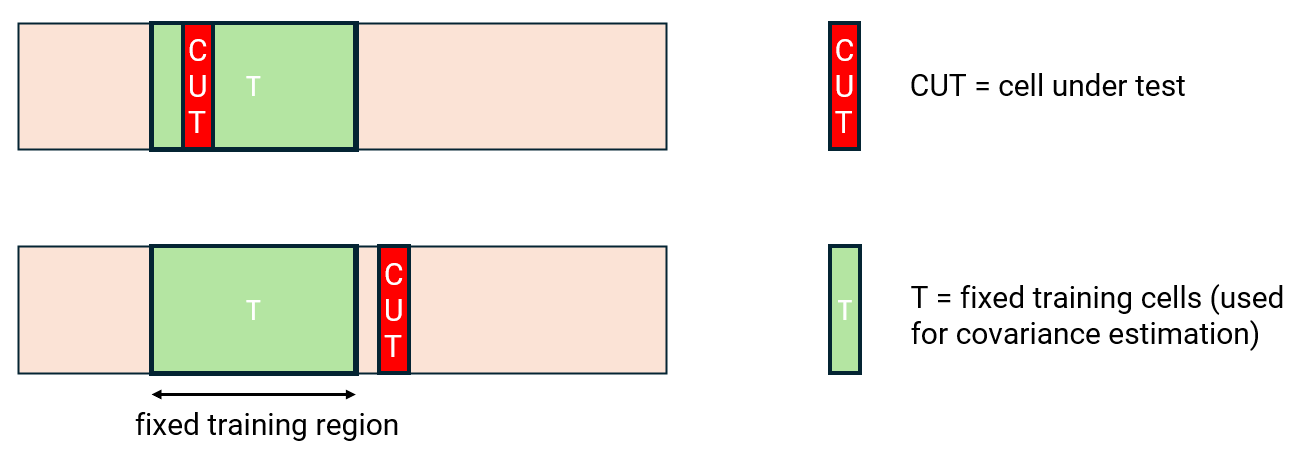
Fixed Training Cells Approach

The range cells are divided into fixed, non-overlapping training regions. A single covariance matrix is computed for each region and reused for all associated CUTs. This method is simple and can make the ACE detector run fast because less covariance matrix inversion is computed. However, there are two major limitations for this method. First, training cells may overlap with CUTs, leading to biased estimates if target signals leak into training data. Second, distant training cells might not accurately represent local noise statistics near the CUT, especially in heterogeneous environments.

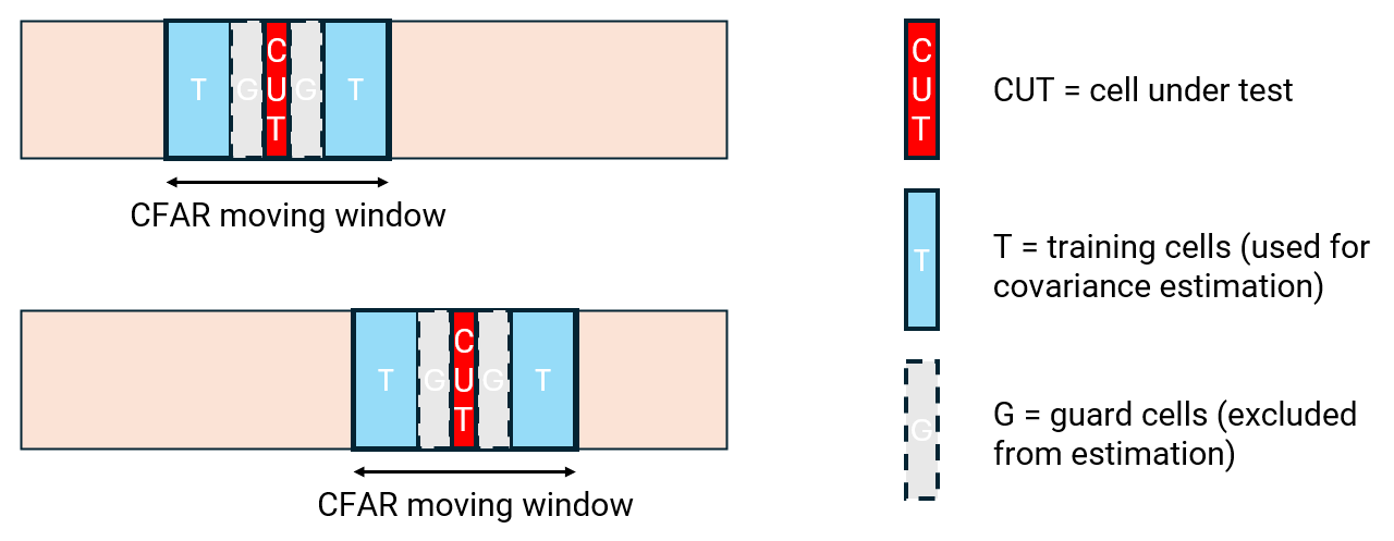
CFAR-Like Sliding Window Weight Approach

Training cells dynamically adjust with the CUT position, maintaining a symmetric window around it. Guard cells isolate the CUT from training regions to prevent contamination. This method ensures target-free training and the proximity of training cells to the CUT improves noise covariance accuracy. However, this method leads to higher computational cost in the ACE detector due to repeated covariance updates for each CUT.

% Choose training data selection method
trainingDataSelectMethod = "CFAR";
numTrainingCells = 80;      % Training cells for covariance estimation
if strcmp(trainingDataSelectMethod,"CFAR") % CFAR-like sliding window weight training cell selection
    % Get training indices using CFAR method
    numGuardCells = 4;   % Guard cells around target
    trainingIndices = helperGetCFARTrainingIndices(cutIndices, numSamples, ...
        numTrainingCells, numGuardCells);

    % Preallocate training data [numTrainingCells x spaceTimeDim x numCutCells]
    trainingData = zeros(numTrainingCells, spaceTimeDim, numCutCells);

    % Extract training data for each CUT
    for cellIdx = 1:numCutCells
        % Extract training data for current looking cell
        trainingIdx = trainingIndices(:, cellIdx);
        trainingData(:, :, cellIdx) = reshape(receivePulse(trainingIdx, :, :), ...
            numTrainingCells, spaceTimeDim);
    end
else % Fixed training cell selection
    % Get fixed training indices
    startCellIdx = tgtCellIndex - ceil(numTrainingCells/2); %#ok<UNRCH>
    trainingIdx = helperGetFixedTrainingIndices(startCellIdx, numSamples, numTrainingCells); 

    % Extract fixed training data [numTrainingCells x spaceTimeDim]
    trainingData = reshape(receivePulse(trainingIdx, :, :), ...
            numTrainingCells, spaceTimeDim);
end

Covariance Estimation

The accuracy of adaptive detection hinges on precise noise covariance estimation. While training data selection determines which samples are used, the choice of estimator governs how these samples are transformed into statistical knowledge. Below we compare two covariance estimators.

Sample Covariance Matrix (SCM)

$${\underset{}{\overset{ˆ}{M}}}_{SCM}=\frac{1}{K}\sum _{k=1}^K{y}_k{y}_k^H$$

The SCM covariance estimator assumes the training data and CUT share identical covariance. SCM is the maximum likelihood estimator for homogeneous Gaussian noise. However, its performance degrades in heterogeneous environments (e.g., when clutter and interference power vary across range cells).

Normalized SCM (NSCM)

$${\underset{}{\overset{ˆ}{M}}}_{NSCM}=\frac{N}{K}\sum _{k=1}^K\frac{y_k{y}_k^H}{y_k^H{y}_k},$$

where $$N$$ is the dimension of training data $$y_k$$. The NSCM is a more robust covariance estimator for the partially homogeneous environment or compound-Gaussian environment.

• In the partially homogeneous environment, the training data $$y$$ and the CUT data $$y_k,k=1,\dots ,K,$$ share covariance structure up to an unknown scaling factor $$\rho$$ (i.e., $$\text{cov}(y)=M,\text{cov}(y_k)=\rho M$$).

• In the compound-Gaussian environment, the noise in a cell can be modeled as $$c=\sqrt{\tau }x$$, where $$\tau$$ (texture) is a random power level, and $$x$$ (speckle) is a zero-mean complex Gaussian with covariance $$M$$.

In this example, the coexistence of angle-localized interference and Doppler-spread clutter creates a heterogeneous noise field. The NSCM's normalization inherently compensates for power variations across range cells, yielding more accurate covariance estimates and superior ACE detection performance compared to SCM.

When the training data is limited (e.g., $$K<2N$$) or heterogeneous noise exists (e.g., clutter/interference power variations), the covariance matrix estimate can be ill-conditioned. In this case, the covariance matrix estimate can be enhanced via shrinkage-based diagonal loading approach.

% Configure covariance matrix estimation method
covEstimationMethod = "NSCM";
covEstimator = HelperCovarianceEstimator(Method = covEstimationMethod,...
    DiagonalLoading = 'Shrinkage');

% Obtain covariance matrix estimate
numTrainingWindows = size(trainingData,3);
nCov = zeros(spaceTimeDim, spaceTimeDim, numTrainingWindows);
for m = 1:numTrainingWindows
    nCov(:,:,m) = covEstimator(trainingData(:,:,m));
end

ACE Detection

Configure the parameters of the ACE detector: the probability of false alarm $$P_{fa}$$ and the number of training data $$K$$. These parameters are used for setting ACE detection threshold $$\gamma$$.

% Configure ACE detectors
pfa = 1e-6; % Probability of false alarm
aceDetector = HelperACEDetector(ProbabilityFalseAlarm = pfa, ...
    NumTrainingSamples = numTrainingCells);

The ACE detector evaluates each range CUT by computing detection statistics $${\Lambda }_{\text{ACE}}(y,\underset{}{\overset{ˆ}{M}})$$ across all angle-Doppler bins. For every angle-Doppler bin, it applies:

1. The space-time steering vector $$s$$ corresponding to that specific angle-Doppler combination;

2. The estimated noise covariance matrix $$\underset{}{\overset{ˆ}{M}}$$ for interference and clutter suppression.

% Run ACE detection
[detectResult,detectStat,detectTh] = ...
    aceDetector(cutData,stSteeringVecs,nCov);

% Convert [(numDopBins*numAngBins) x numCutCells] to [numDopBins x numAngBins x numCutCells]
detectionResult3d = helperReshapeDetectionData(detectResult, ...
    numDopBins, numAngBins, numCutCells);
detectionStat3d = helperReshapeDetectionData(detectStat, ...
    numDopBins, numAngBins, numCutCells);

Detection Result Display

Display the 2D ACE detection result at the CUT with the target.

checkCellIdx = 1;
detectionResult2d = detectionResult3d(:,:,checkCellIdx);
detectionStat2d = detectionStat3d(:,:,checkCellIdx);
helperPlotACEDetectionResult(angGrid, dopGrid, detectionStat2d, detectionResult2d)

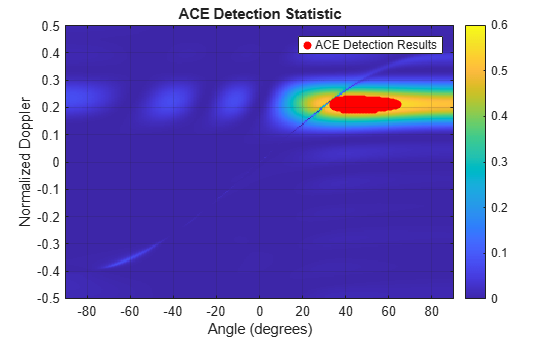
This plot shows that the ACE detector can successfully identify potential targets while suppressing interference and clutter signals.

Summary

In this example, you learned how to use the Adaptive Coherence Estimator (ACE) detector to detect targets under heterogeneous clutter and interference environment. You learned 2 different ways of selecting training data taking into consideration computational time and accuracy. You also learned how to estimate noise covariance given limited and heterogeneous data samples.

Reference

[1] Fulvio Gini and Maria Greco, "Covariance matrix estimation for CFAR detection in correlated heavy tailed clutter." Signal Processing, 2002.

[2] F. Pascal, P. Forster, J. -P. Ovarlez and P. Larzabal, "Performance Analysis of Covariance Matrix Estimates in Impulsive Noise," IEEE Transactions on Signal Processing, vol. 56, no. 6, pp. 2206-2217, June 2008.

[3] Antonio De Maio and Maria Greco, Modern Radar Detection Theory, Chapter 8, pp. 295-332, 2016.

[4] J. Liu, H. Li and B. Himed, "Threshold Setting for Adaptive Matched Filter and Adaptive Coherence Estimator," IEEE Signal Processing Letters, vol. 22, no. 1, pp. 11-15, Jan. 2015.

[5] L. T. McWhorter, L. L. Scharf and L. J. Griffiths, "Adaptive coherence estimation for radar signal processing," Conference Record of The Thirtieth Asilomar Conference on Signals, Systems and Computers, Pacific Grove, CA, USA, pp. 536-540 vol.1, 1996.