Integrated Sensing and Communication Using 5G Waveform

Since R2025a

This example demonstrates integrated sensing and communication capabilities (ISAC) of a 5G New Radio (NR) waveform. It simulates data frame transmissions through the physical downlink shared channel (PDSCH) of a 5G NR link and shows how the channel matrix estimates obtained from the received frames can be processed to extract radar measurements of moving scatterers present in the channel.

Introduction

The core concept of the Integrated Sensing and Communication (ISAC) is the utilization of the same hardware and frequency spectrum to perform both communication and sensing functions. Recent research has explored various ISAC approaches, ranging from the joint design of novel dual-function systems to enabling sensing capabilities within existing wireless networks. The latter approach is particularly attractive as it leverages existing equipment and network infrastructure. Incorporating sensing into next-generation wireless networks, such as beyond 5G (B5G) and 6G, not only would help alleviate electromagnetic spectrum congestion but also enable a range of emerging applications. These include high-accuracy localization and tracking, as well as human activity recognition.

This example illustrates how sensing can be effectively accomplished using a 5G NR waveform, as defined by the 3GPP NR standard. Channel matrix estimates obtained from received PDSCH frames inherently capture information about the time delays and Doppler shifts experienced by the transmitted waveform as it travels to the receiver. By processing this information, in a manner akin to standard radar data cube techniques, these time delays and Doppler shifts can be translated into the positions and velocities of the corresponding scatterers, thereby forming radar detections

The example begins by defining an ISAC scenario with a single transmitter and a single receiver, where the transmitter represents a base station and the receiver models user equipment. It then configures the transmitted 5G NR waveform, illustrating that the selection of demodulation reference signal (DM-RS) parameters is directly related to the desired sensing performance. The example proceeds by simulating the propagation of PDSCH frames through a scattering MIMO channel. For each received frame, the channel matrix is estimated and then processed to detect moving scatterers present in the channel. The example demonstrates that from the sensing perspective, the modeled 5G link is a bistatic radar capable of measuring bistatic range and angle-of-arrival of the targets. Finally, these measurements are passed to a tracking algorithm to form target tracks and estimate target positions and velocities in Cartesian coordinates.

ISAC Scenario

Consider a 5G NR link operating at a frequency of 60 GHz.

rng('default');                                            % Set the random number generator for reproducibility
carrierFrequency = 60e9;                                   % Carrier frequency (Hz)
wavelength = freq2wavelen(carrierFrequency);

Let the transmitter (gNodeB) be located at the origin.

txPosition = [0; 0; 0];                                    % Base station location

Create a transmitter object and set the transmit power to 46 dBm.

txPower = 46;                                             % dBm
transmitter = phased.Transmitter('PeakPower', db2pow(txPower-30), 'Gain', 0);

Let the transmitter have a uniform linear array (ULA) of eight isotropic antenna elements spaced half a wavelength apart.

numTxAntennas = 8;                                         % Number of antenna elements at the Tx array 
element = phased.IsotropicAntennaElement('BackBaffled', true);
txArray = phased.ULA(numTxAntennas, wavelength/2, 'Element', element);

Point the transmit array normal along the x-axis.

txOrientationAxes = eye(3);                                % Tx array orientation

Let the receiver (user equipment) be located some distance away from the transmitter.

rxPosition = [50; 60; 0];                                  % User equipment location

Create a receiver object. Set the noise figure to 5 dB and the reference temperature to 290.

receiver = phased.Receiver('AddInputNoise', true, 'Gain', 0, 'NoiseMethod', 'Noise figure',...
    'NoiseFigure', 5, 'ReferenceTemperature', 290);

Let the receiver have a uniform linear array (ULA) of eight isotropic antenna elements spaced half a wavelength apart.

numRxAntennas = 8;                                         % Number of antenna elements at the Rx array
rxArray = phased.ULA(numRxAntennas, wavelength/2, 'Element', element);

Point the receive array normal along the negative y-axis.

rxOrientationAxes = rotz(-90);                             % Rx array orientation

Use the helperGenerateStaticScatterers helper function to generate positions and reflection coefficients of 40 point scatterers.

regionOfInterest = [0 120; -80 80];                        % Region of interest
numScatterers = 40;                                        % Number of scatterers distributed with the region of interest

% Randomly distributed scatterers
[scatterers.Positions, scatterers.ReflectionCoefficients] = ...
    helperGenerateStaticScatterers(numScatterers, regionOfInterest);

Assume the generated scatterers are static.

scatterers.Velocities = zeros(size(scatterers.Positions));

Use the helperGetTargetTrajectories helper function to generate two straight line constant speed trajectories for two moving scatterers. These scatterers are the targets of interest for the sensing function.

targets.Trajectories = helperGetTargetTrajectories();

ans=2×5 table
    Trajectory    Start Position [x, y]    End Position [x, y]    Length (m)    Speed (m/s)
    __________    _____________________    ___________________    __________    ___________

       "1"              {[25 -5]}               {[40 30]}           38.079        9.5197   
       "2"              {[70 30]}               {[80 10]}           22.361        5.5902   

% Target reflection coefficients
numTargets = numel(targets.Trajectories);
targets.ReflectionCoefficients = exp(1i*(2*pi*rand(1, numTargets)));

Use phased.ScatteringMIMOChannel object to model the propagation channel between the transmitter and the receiver.

channel = phased.ScatteringMIMOChannel('CarrierFrequency', carrierFrequency, 'TransmitArray', txArray,...
    'TransmitArrayPosition', txPosition, 'ReceiveArray', rxArray, 'ReceiveArrayPosition', rxPosition,...
    "TransmitArrayOrientationAxes", txOrientationAxes, "ReceiveArrayOrientationAxes", rxOrientationAxes,... , 
    'SimulateDirectPath', true, 'ScattererSpecificationSource', 'Input Port', ...
    'ChannelResponseOutputPort',true,'Polarization','None');

Visualize the scenario using the helperVisualizeScatteringMIMOChannel helper function.

helperVisualizeScatteringMIMOChannel(channel, scatterers.Positions, targets.Trajectories);
title('ISAC Scenario');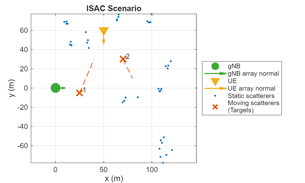

Note, that from the sensing perspective, in this scenario the transmitter and the receiver form a bistatic pair.

5G Waveform Configuration

Set system parameters for 5G NR. Let the channel bandwidth be 50 MHz.

channelBandwidth = 50;                                     % MHz - transmission bandwidth and guardbands

Set the bandwidth occupancy. This is the ratio between the transmission bandwidth and channel bandwidth. A lower bandwidth occupancy increases the size of guardbands, reducing spectral emissions at the cost of reduced spectral efficiency.

bandwidthOccupancy = 0.9;                                  % Ratio of transmission bandwidth to channel bandwidth

Let the subcarrier spacing be 60 kHz.

subcarrierSpacing = 60;                                    % Subcarrier spacing (kHz)

Use the helperGet5GWaveformConfiguration to create a 5G waveform configuration.

waveformConfig = helperGet5GWaveformConfiguration(channelBandwidth, bandwidthOccupancy, subcarrierSpacing);
waveformInfo = nrOFDMInfo(waveformConfig.Carrier)

waveformInfo = struct with fields:
                   Nfft: 1024
             SampleRate: 61440000
    CyclicPrefixLengths: [104 72 72 72 72 72 72 72 72 72 72 72 72 72 72 72 72 72 72 72 72 72 72 72 72 72 72 72 104 72 72 72 72 72 72 72 72 72 72 72 72 72 72 72 72 72 72 72 72 72 72 72 72 72 72 72]
          SymbolLengths: [1128 1096 1096 1096 1096 1096 1096 1096 1096 1096 1096 1096 1096 1096 1096 1096 1096 1096 1096 1096 1096 1096 1096 1096 1096 1096 1096 1096 1128 1096 1096 1096 1096 1096 1096 1096 1096 1096 1096 1096 1096 1096 … ] (1×56 double)
              Windowing: 36
           SymbolPhases: [0 0 0 0 0 0 0 0 0 0 0 0 0 0 0 0 0 0 0 0 0 0 0 0 0 0 0 0 0 0 0 0 0 0 0 0 0 0 0 0 0 0 0 0 0 0 0 0 0 0 0 0 0 0 0 0]
         SymbolsPerSlot: 14
       SlotsPerSubframe: 4
          SlotsPerFrame: 40

transmissionBandwidth = subcarrierSpacing*1e3*waveformConfig.Carrier.NSizeGrid*12; % Bandwidth of resource blocks in Hz
fprintf("Transmission bandwidth: %d MHz\n",transmissionBandwidth);

Transmission bandwidth: 44640000 MHz

Set the channel sample rate to the waveform's sample rate.

channel.SampleRate = waveformInfo.SampleRate;

PDSCH frames include DM-RS signals that help the receiver estimate the channel characteristics. The communication function uses this information to correctly demodulate the transmitted data. The sensing function can use the same information to estimate positions and velocities of the scatterers in the channel. The configuration of DM-RS pilot signals will directly influence the sensing performance. See NR PDSCH Resource Allocation and DM-RS and PT-RS Reference Signals (5G Toolbox) example to learn more about different DM-RS configurations.

Set the DM-RS parameters.

waveformConfig.PDSCH.DMRS.DMRSTypeAPosition = 2;           % Mapping type A only. First DM-RS symbol position is 2
waveformConfig.PDSCH.DMRS.DMRSLength = 1;                  % Single-symbold DM-RS
waveformConfig.PDSCH.DMRS.DMRSAdditionalPosition = 2;      % Additional DM-RS symbol positions (max range 0...3)
waveformConfig.PDSCH.DMRS.NumCDMGroupsWithoutData = 1;     % Number of CDM groups without data
waveformConfig.PDSCH.DMRS.DMRSConfigurationType = 1;       % DM-RS configuration type (1,2)

Visualize one resource block of the configured resource grid.

resourceGrid = nrResourceGrid(waveformConfig.Carrier, waveformConfig.PDSCH.NumLayers);
ind = nrPDSCHDMRSIndices(waveformConfig.Carrier, waveformConfig.PDSCH);
resourceGrid(ind) = nrPDSCHDMRS(waveformConfig.Carrier, waveformConfig.PDSCH);

helperVisualizeResourceGrid(abs(resourceGrid(1:12,1:14,1)));
title({'PDSCH DM-RS Resource Elements in the Carrier Resource Grid', '(single resource block)'});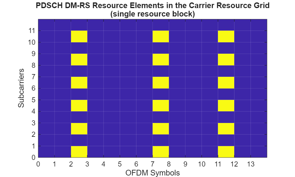

The density of pilot signals in the time domain determines the maximum Doppler shift that can be measured unambiguously, without causing aliasing. In the configured PDSCH frame, the maximum separation between pilot signals in the time domain is ${\mathit{M}}_{\mathit{t}}$ = 5 symbols. The corresponding maximum unambiguous Doppler shift can be computed using the formula

$${\mathit{f}}_{\mathrm{Dmax}}\le \frac{1}{2{\mathit{M}}_{\mathit{t}}{\mathit{T}}_{\mathrm{OFDM}}}$$

where ${\mathit{T}}_{\mathrm{OFDM}}$is the symbol duration.

% Compute maximum pilot signal separation in time
[~,pdschInfo] = nrPDSCHIndices(waveformConfig.Carrier,waveformConfig.PDSCH);
Mt = max(diff(pdschInfo.DMRSSymbolSet));

% Duration of an OFDM symbol in seconds
ofdmSymbolDuration = mode(waveformInfo.SymbolLengths)/waveformInfo.SampleRate;

maxDoppler = 1/(2*Mt*ofdmSymbolDuration);
fprintf('Maximum unambiguous Doppler shift: %.2f kHz\n', maxDoppler*1e-3);

Maximum unambiguous Doppler shift: 5.61 kHz

Compute the corresponding maximum velocity and compare it to the maximum ground speeds of the targets in the considered ISAC scenario.

maxVelocity = dop2speed(maxDoppler, wavelength)/2;
fprintf('Maximum unambiguous velocity: %.2f m/s\n', maxVelocity);

Maximum unambiguous velocity: 14.00 m/s

The velocities of the targets in the scenario are within the maximum unambiguous velocity.

Similarly, the density of pilot signals in the frequency domain determines the maximum time delay that can be measured without causing aliasing. In the frequency domain the pilot signals repeat every ${\mathit{M}}_{\mathit{f}}$= 2 subcarriers. The corresponding maximum unambiguous time delay can be computed using formula

$${\tau }_{\max }\le \frac{1}{2{\mathit{M}}_{\mathit{f}}\Delta \mathit{f}}$$

where $\Delta \mathit{f}$is the subcarrier spacing.

% Compute pilot signal separation in frequency
Mf = min(diff(waveformConfig.PDSCH.DMRS.DMRSSubcarrierLocations));
maxDelay = 1/(2*Mf*subcarrierSpacing*1e3);
fprintf('Maximum time delay: %.2fe-6 s\n', maxDelay*1e6);

Maximum time delay: 4.17e-6 s

Compute the corresponding maximum range.

maxRange = time2range(maxDelay);
fprintf('Maximum unambiguous range: %.2f m\n', maxRange);

Maximum unambiguous range: 624.57 m

All targets in the scenario are well within the maximum unambiguous range.

Finally, the transmission bandwidth determines the range resolution.

% Range resolution
rangeResolution = bw2rangeres(transmissionBandwidth);
fprintf('Range resolution: %.2f m\n', rangeResolution);

Range resolution: 3.36 m

This resolution is sufficient for resolving the targets in the scenario.

Channel Simulation and Sensing Data Processing

This example simulates the transmission of 10 PDSCH frames, with each frame transmitted 0.4 seconds apart, covering a total time span of 3.6 seconds. This approach is necessary to effectively demonstrate changes in the target's positions. Simulating every frame within this time interval would be computationally prohibitive. However, it is assumed that the 5G NR link continues to operate normally between the simulated frames.

% Number of PDSCH frames to simulate
numSensingFrames = 10;

% Time step between simulated PDSCH frames (s)
dt = 0.4;

% Simulation times
t = (0:numSensingFrames-1)*dt;

A channel matrix estimate is obtained from each PDSCH frame transmission. The channel matrix has dimensions $\mathit{K}\times \mathit{N}\times \mathit{R}\times \mathit{P}$, where $\mathit{K}$ is the number of subcarriers, $\mathit{N}$ is the total number of OFDM symbols in one frame, $\mathit{R}$is the number of receive antennas, and $\mathit{P}$ is the number of reference signal ports. In this example the base station does not perform any beamforming, thus $\mathit{P}$ is equal to the number of transmit antennas. The channel matrix estimate can be viewed as a radar data cube, with each dimension representing:

• Subcarrier dimensions as the range (fast-time),

• Symbol dimension as the slow-time,

• Receive antenna dimension as the angle-of-arrival (AoA),

• Reference signal ports dimension as the angle-of-departure (AoD).

Each dimension of the channel matrix estimate can be processed separately. The results can then be non-coherently integrated over the slow-time and AoD dimensions to produce a range-AoA map, which can be used to estimate the positions of targets.

To perform this processing define a grid of AoAs and compute the corresponding steering vectors.

numAoA = ceil(2*pi*numRxAntennas);                         % AoA grid size
aoaGrid = linspace(-90, 90, numAoA);                       % AoA grid

% Receive array steering vectors
rxSteeringVector = phased.SteeringVector(SensorArray=channel.ReceiveArray);
rxsv = rxSteeringVector(carrierFrequency, aoaGrid);

Define a grid of AoDs and compute the corresponding steering vectors.

numAoD = ceil(2*pi*numTxAntennas);                         % AoD grid size
aodGrid = linspace(-90, 90, numAoD);                       % AoD grid

% Transmit array steering vectors
txSteeringVector = phased.SteeringVector(SensorArray=channel.TransmitArray);
txsv = txSteeringVector(carrierFrequency, aodGrid);

Define a bistatic range grid and the corresponding fast-time steering vectors.

% Limit the maximum bistatic range of interest to 100 meters
maxRange = 100;
rangeGrid = -20:rangeResolution/2:maxRange;             % Bistatic range grid
numRange = numel(rangeGrid);                            % Bistatic range grid size

% Baseline distance between Tx and Rx
baseline = vecnorm(txPosition - rxPosition);

% Fast-time steering vectors 
rangeFFTBins = (rangeGrid+baseline)/(2*rangeResolution);
numSubcarriers = waveformConfig.Carrier.NSizeGrid*12;
k = (0:numSubcarriers-1).';
rngsv = (exp(2*pi*1i*k*rangeFFTBins/numSubcarriers)/numSubcarriers);

Set up a 2-D constant false alarm rate (CFAR) detector to process bistatic range-AoA maps. Determine the CFAR guard band size based on the range and angle resolution.

% Number of guard cells in range
numGuardCellsRange = ceil(rangeResolution/(rangeGrid(2)-rangeGrid(1))) + 1;

% Resolution in AoA domain
aoaResolution = ap2beamwidth((numRxAntennas-1)*channel.ReceiveArray.ElementSpacing, wavelength);

% Number of guard cells in AoA
numGuardCellsAoA = ceil(aoaResolution/(aodGrid(2)-aodGrid(1))) + 1;

% Create a 2-D CFAR detector
cfar2D = phased.CFARDetector2D('GuardBandSize',[numGuardCellsRange numGuardCellsAoA], 'TrainingBandSize', [4 6],...
    'ProbabilityFalseAlarm', 1e-3, 'OutputFormat', 'CUT result', 'ThresholdOutputPort', false);

% Compute indices of the cells under test
offsetIdxs = cfar2D.TrainingBandSize + cfar2D.GuardBandSize;

rangeIdxs = offsetIdxs(1)+1:numel(rangeGrid)-offsetIdxs(1);    
angleIdxs = offsetIdxs(2)+1:numel(aoaGrid)-offsetIdxs(2);

[sumRangeIdxs, aoaIdxs] = meshgrid(rangeIdxs, angleIdxs);
cutidx = [sumRangeIdxs(:).'; aoaIdxs(:).'];

The CFAR algorithm can produce multiple detections around the true target positions. These detections are typically clustered together to obtain a single detection. Create a DBSCAN clusterer object.

clusterer = clusterDBSCAN();

Use the helperConfigureTracker helper function to create a target tracking object. The returned tracker is configured to perform tracking using bistatic range and angle of arrival measurements. The tracker's state vector is in Cartesian coordinates. Thus, the tracker not only improves target position estimates but also estimates target velocities.

tracker = helperConfigureTracker(txPosition, rxPosition, txOrientationAxes, rxOrientationAxes, rangeResolution, aoaResolution);

% Preallocate space to store estimated target state vectors [x; vx; y; vy]
% Preallocate space for 10 tracks
targetStateEstimates = zeros(4, numSensingFrames, 10);
trackIDs = [];

To generate visualizations showing the ISAC scenario together, the true target positions, target detections, and tracks, set generateVisualizations to true.

% Produce visualizations
generateVisualizations = false;

if generateVisualizations
    scenarioCFARResultsFigure = figure;
    tl = tiledlayout(scenarioCFARResultsFigure, 1, 2, 'Padding', 'tight', 'TileSpacing', 'tight');

Use the helperTheaterPlotter to visualize the scenario, target trajectories, detections, and tracks.

    scenarioPlotter = helperTheaterPlotter(tl);
    scenarioPlotter.plotTxAndRx(txPosition, rxPosition);
    scenarioPlotter.plotTrajectories(targets.Trajectories, t);
    scenarioPlotter.plotScatterers(scatterers.Positions);
    title(scenarioPlotter, 'ISAC Scenario');

Use helperCFARResultsVisualizer to visualize CFAR results.

    cfarResultsVisualizer = helperCFARResultsVisualizer(tl);
    xlabel(cfarResultsVisualizer, 'AoA (degrees)');
    ylabel(cfarResultsVisualizer, 'Bistatic Range (m)');
    title(cfarResultsVisualizer, 'CFAR Results');
end

Run the simulation transmitting and processing one PDSCH frame at a time.

% Number of symbols per frame
numSymbolsPerFrame = waveformInfo.SlotsPerFrame*waveformInfo.SymbolsPerSlot;

% Transmit and process one PDSCH frame at a time
for i = 1:numSensingFrames
    fprintf('\nSimulating frame at time %g s\n', t(i));
    
    % helperSimulateLinkSingleFrame returns a 4-D matrix 
    % numSubcarriers x numSymbolsPerFrame x numRxAntennas x numTxAntennas
    sensingCSI = helperSimulateLinkSingleFrame(transmitter, receiver, channel, waveformConfig, scatterers, targets, t(i));

    % Reset the channel between PDSCH frame transmissions
    reset(channel);

    % To filter the static scatterers out, put a zero in the first Doppler
    % bin
    X = fft(sensingCSI, [], 2);
    X(:, 1, :, :) = 0;
    x = ifft(X, [], 2);

    % Process data cube along the AoD dimension
    x = permute(x, [4 1 3 2]);
    x = txsv'*reshape(x, numTxAntennas, []);

    % Process data cube along the range dimension
    x = permute(reshape(x, numAoA, numSubcarriers, numRxAntennas, numSymbolsPerFrame), [2 3 1 4]);
    x = rngsv.'*reshape(x, numSubcarriers, []);

    % Process data cube along the AoA dimension
    x = permute(reshape(x, numRange, numRxAntennas, numAoD, numSymbolsPerFrame), [2 1 3 4]);
    x = rxsv'*reshape(x, numRxAntennas, []);

    % Average over AoDs and symbols
    x = reshape(x, numAoA, numRange, []);
    sumRangeAoAMap = sqrt(sum(abs(x).^2, 3)).';

    % Perform 2-D CFAR detection over range-AoA map
    cutResult = cfar2D(sumRangeAoAMap, cutidx);
    detectionIdxs = cutidx(:, cutResult);
    detectionValues = [rangeGrid(detectionIdxs(1,:)); aoaGrid(detectionIdxs(2,:))];    

    % Cluster CFAR detections
    [~, clusterids] = clusterer(detectionValues.');
    uniqClusterIds = unique(clusterids);

    % Loop over detection clusters, and for each cluster find a
    % center
    m = numel(uniqClusterIds);
    clusteredDetections = zeros(2, m);

    for j = 1:m
        idxs = clusterids == uniqClusterIds(j);
        d = detectionValues(:, idxs);

        % Represent a cluster of detections with its center 
        clusteredDetections(:, j) = mean(d, 2);
    end

    % Format detections so that they can be processed by the tracker
    detections = helperFormatDetectionsForTracker(clusteredDetections, t(i), rangeResolution, aoaResolution);
    
    % Pass detections to the tracker
    tracks = tracker(detections);

    % Store target state estimates
    for it = 1:numel(tracks)
        id = tracks(it).TrackID;
        trackIDs = union(trackIDs, id);        
        targetStateEstimates(:, i, id) = tracks(it).State;
    end    
    
    % Visualization
    if generateVisualizations
        % Plot true target positions
        targetPositions = zeros(numTargets, 3);
        for it = 1:numTargets
            targetPositions(it, :) = lookupPose(targets.Trajectories{it}, t(i));
        end
        scenarioPlotter.plotTargetPositions(targetPositions);
       
        % Plot target positions estimated from the detections
        measuredPositions = helperGetCartesianMeasurement(clusteredDetections, txPosition, rxPosition, rxOrientationAxes);
        scenarioPlotter.plotDetections(measuredPositions);
        scenarioPlotter.plotTracks(tracks);
    
        % Visualize CFAR results 
        [trueRrx, trueAoA] = rangeangle(targetPositions.', rxPosition, rxOrientationAxes);
        [trueRtx, trueAoD] = rangeangle(targetPositions.', txPosition, txOrientationAxes);
        trueBistaticRange = trueRrx + trueRtx - baseline;
    
        cfarResultsVisualizer.plotCFARImage(aoaGrid, rangeGrid, sumRangeAoAMap);
        cfarResultsVisualizer.plotTruth([trueBistaticRange; trueAoA(1, :)]);
        cfarResultsVisualizer.plotClusteredDetections(clusteredDetections);

        sgtitle(scenarioCFARResultsFigure, sprintf('Frame %d, Simulation Time %.1f s', i, t(i)), 'FontSize' ,10);
    end
end

Simulating frame at time 0 s

Throughput(Mbps) for 1 frame(s) = 1.7928
Throughput(%) for 1 frame(s) = 100.0000

Simulating frame at time 0.4 s

Throughput(Mbps) for 1 frame(s) = 1.7928
Throughput(%) for 1 frame(s) = 100.0000

Simulating frame at time 0.8 s

Throughput(Mbps) for 1 frame(s) = 1.7928
Throughput(%) for 1 frame(s) = 100.0000

Simulating frame at time 1.2 s

Throughput(Mbps) for 1 frame(s) = 1.7928
Throughput(%) for 1 frame(s) = 100.0000

Simulating frame at time 1.6 s

Throughput(Mbps) for 1 frame(s) = 1.7928
Throughput(%) for 1 frame(s) = 100.0000

Simulating frame at time 2 s

Throughput(Mbps) for 1 frame(s) = 1.7928
Throughput(%) for 1 frame(s) = 100.0000

Simulating frame at time 2.4 s

Throughput(Mbps) for 1 frame(s) = 1.7928
Throughput(%) for 1 frame(s) = 100.0000

Simulating frame at time 2.8 s

Throughput(Mbps) for 1 frame(s) = 1.7928
Throughput(%) for 1 frame(s) = 100.0000

Simulating frame at time 3.2 s

Throughput(Mbps) for 1 frame(s) = 1.7928
Throughput(%) for 1 frame(s) = 100.0000

Simulating frame at time 3.6 s

Throughput(Mbps) for 1 frame(s) = 1.7928
Throughput(%) for 1 frame(s) = 100.0000

The simulation results show that radar detections in bistatic range-AoA space can be successfully formed by processing the channel matrix estimates. These detections are close to the true target positions. Subsequently, the tracker utilizes these detections to estimate targets' states, which consist of positions and velocities in Cartesian coordinates.

Use helperPlotSpeedEstimationResults helper function to compare target speed and heading estimates based on the tracker outputs with the true values.

helperPlotSpeedEstimationResults(t, targets.Trajectories, targetStateEstimates, trackIDs)

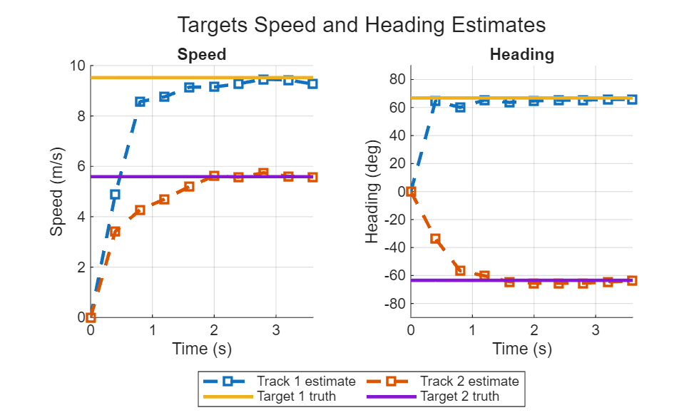
Notice that the tracker requires at least two initial detections to initiate a track and start computing velocities. This is why it can take several track updates before the speed and the heading estimates converge to the true values.

Conclusion

This example demonstrates the sensing capabilities of a 5G NR waveform by illustrating the process of extracting bistatic radar information from the channel matrix estimates obtained during the transmission of PDSCH frames. It discusses the influence of the selected DM-RS parameters on the sensing performance. The example then simulates an ISAC scenario with multiple transmitted PDSCH frames. For each received frame the channel matrix is processed in a manner akin to a radar data cube. Example shows how to set up a signal processing chain for bistatic range and AoA estimation. This processing chain includes computing range and angle responses, followed by CFAR detection and DBSCAN clustering to produce detections. Finally, the detections in bistatic range and AoA space are input into a tracking algorithm, which calculates the targets' positions and velocity estimates in Cartesian coordinates.

Supporting Functions

function tracker = helperConfigureTracker(txPosition, rxPosition, txOrientation, rxOrientation, rangeResolution, aoaResolution)
    % Sensor specification
    sensorSpec = trackerSensorSpec("aerospace", "radar", "bistatic");
    sensorSpec.MeasurementMode = "range-angle";
    sensorSpec.IsReceiverStationary = true;
    sensorSpec.IsEmitterStationary = true;
    sensorSpec.HasElevation = false;
    sensorSpec.HasRangeRate = false;
    sensorSpec.MaxNumLooksPerUpdate = 1;
    sensorSpec.MaxNumMeasurementsPerUpdate = 10;
    sensorSpec.EmitterPlatformPosition = txPosition;
    sensorSpec.EmitterPlatformOrientation = txOrientation.';
    sensorSpec.ReceiverPlatformPosition = rxPosition;
    sensorSpec.ReceiverPlatformOrientation = rxOrientation.';
    sensorSpec.RangeResolution = rangeResolution;
    sensorSpec.AzimuthResolution = aoaResolution;
    sensorSpec.ReceiverFieldOfView = [360 180];
    sensorSpec.EmitterFieldOfView = [360 180];
    sensorSpec.ReceiverRangeLimits = [0 500];
    sensorSpec.EmitterRangeLimits = [0 500];
    sensorSpec.DetectionProbability = 0.9;

    % Target specification
    targetSpec = trackerTargetSpec('custom');
    targetSpec.StateTransitionModel = targetStateTransitionModel('constant-velocity');
    targetSpec.StateTransitionModel.NumMotionDimensions = 2;
    targetSpec.StateTransitionModel.VelocityVariance = 15^2/3*eye(2);
    targetSpec.StateTransitionModel.AccelerationVariance = 0.01^2/3*eye(2);    
    
    tracker = multiSensorTargetTracker(targetSpec,sensorSpec,"jipda"); 
    tracker.ConfirmationExistenceProbability = 0.98; 
    tracker.MaxMahalanobisDistance = 10;
end

function detections = helperFormatDetectionsForTracker(clusteredDetections, currentTime, rangeResoultion, aoaResolution)
    numDetections = size(clusteredDetections, 2);
    detections.ReceiverLookTime = currentTime;
    detections.ReceiverLookAzimuth = 0;
    detections.ReceiverLookElevation = 0;
    detections.EmitterLookAzimuth = 0;
    detections.EmitterLookElevation = 0;
    detections.DetectionTime = ones(1, numDetections) * currentTime;
    detections.Azimuth = clusteredDetections(2, :);
    detections.Range = clusteredDetections(1, :);

    % The measurement accuracy is proportional to the sensor resolution and
    % depends on the SNR.
    detections.AzimuthAccuracy = ones(1, numDetections) * aoaResolution/12;
    detections.RangeAccuracy = ones(1, numDetections) * rangeResoultion/4;    
end

function meascart = helperGetCartesianMeasurement(dets, txPosition, rxPosition, rxOrientationAxes)
    n = size(dets, 2);
    meassph = zeros(3, n);
    meassph(1, :) = dets(2, :);
    meassph(3, :) = dets(1, :);

    meassph = local2globalcoord(meassph, 'ss', [0; 0; 0], rxOrientationAxes);    
    meascart = bistaticposest(meassph(3, :), meassph(1:2, :), eps*ones(1, n), repmat([eps; eps], 1, n),...
        txPosition, rxPosition, 'RangeMeasurement', 'BistaticRange');
end

function trajectories = helperGetTargetTrajectories()

    % Target #1
    waypoints = [25 -5 0;
                 40 30 0];
    timeOfArrival = [0 4];
    traj1 = waypointTrajectory(waypoints,timeOfArrival);

    % Target #2
    waypoints = [70 30 0;
                 80 10 0];

    timeOfArrival = [0 4];
    traj2 = waypointTrajectory(waypoints,timeOfArrival);
    
    trajectories = {traj1, traj2};

    Trajectory = strings(numel(trajectories), 1);
    Speed = zeros(numel(trajectories), 1);
    Length = zeros(numel(trajectories), 1);
    Start = cell(numel(trajectories), 1);
    Stop = cell(numel(trajectories), 1);

    for i = 1:numel(trajectories)
        Trajectory(i) = i;
        Start{i} = trajectories{i}.Waypoints(1, 1:2);
        Stop{i} = trajectories{i}.Waypoints(end, 1:2);
        Length(i) = vecnorm(trajectories{i}.Waypoints(1, :) - trajectories{i}.Waypoints(end, :));
        Speed(i) = max(trajectories{i}.GroundSpeed);
    end

    table(Trajectory, Start, Stop, Length, Speed, 'VariableNames',...
        {'Trajectory', 'Start Position [x, y]', 'End Position [x, y]', 'Length (m)', 'Speed (m/s)'})
end

function helperPlotSpeedEstimationResults(t, trajectories, targetStateEstimates, trackIDs)
    fig = figure;
    tl = tiledlayout(fig, 1, 2);
    speedAxes = nexttile(tl);
    hold(speedAxes, 'on');
    
    xlabel(speedAxes, 'Time (s)');
    ylabel(speedAxes, 'Speed (m/s)');
    grid(speedAxes, 'on');
    title(speedAxes, 'Speed');
    xlim(speedAxes, [t(1) t(end)]);
    lgd = legend(speedAxes, 'Location', 'southeast', 'Orientation', 'horizontal', 'NumColumns', 2);
    lgd.Layout.Tile = 'south';
    
    headingAxes = nexttile(tl);
    hold(headingAxes, 'on');
    xlabel(headingAxes, 'Time (s)');
    ylabel(headingAxes, 'Heading (deg)');
    grid(headingAxes, 'on');
    title(headingAxes, 'Heading');
    ylim(headingAxes, [-90 90]);    
    xlim(headingAxes, [t(1) t(end)]);

    sgtitle(fig, 'Targets Speed and Heading Esimates')
    
    for it = 1:numel(trackIDs)
        id = trackIDs(it);
        vx = targetStateEstimates(2, :, id);
        vy = targetStateEstimates(4, :, id);
    
        speedEstimate = sqrt(vx.^2 + vy.^2);
        headingEstimate = atan2d(vy, vx);
        plot(speedAxes, t, speedEstimate, 's--', 'LineWidth', 2, 'DisplayName', sprintf('Track %d estimate', trackIDs(it)));
        plot(headingAxes, t, headingEstimate, 's--', 'LineWidth', 2);
    end
    
    for it = 1:numel(trajectories)
        [~, ~, velocity] = lookupPose(trajectories{it}, t);
        trueSpeed = sqrt(velocity(:, 1).^2 + velocity(:, 2).^2);
        trueHeading = atan2d(velocity(:, 2), velocity(:, 1));
        
        plot(speedAxes, t, trueSpeed, '-', 'LineWidth', 2, 'DisplayName', sprintf('Target %d truth', it));
        plot(headingAxes, t, trueHeading, '-', 'LineWidth', 2);
    end
end