MUSIC Super-Resolution DOA Estimation
MUltiple SIgnal Classification (MUSIC) is a high-resolution direction-finding algorithm based on the eigenvalue decomposition of the sensor covariance matrix observed at an array. MUSIC belongs to the family of subspace-based direction-finding algorithms.
Signal Model
The signal model relates the received sensor data to the signals emitted by the source. Assume that there are D uncorrelated or partially correlated signal sources, sd(t). The sensor data, xm(t), consists of the signals, as received at the array, together with noise, nm(t). A sensor data snapshot is the sensor data vector received at the M elements of an array at a single time t.
x(t) is an M-by-1 vector of received snapshot of sensor data which consist of signals and additive noise.
A is an M-by-D matrix containing the arrival vectors. An arrival vector consists of the relative phase shifts at the array elements of the plane wave from one source. Each column of A represents the arrival vector from one of the sources and depends on the direction of arrival, θd. θd is the direction of arrival angle for the dth source and can represents either the broadside angle for linear arrays or the azimuth and elevation angle for planar or 3D arrays.
s(t) is a D-by-1 vector of source signal values from D sources.
n(t) is an M-by-1 vector of sensor noise values.
An important quantity in any subspace method is the sensor covariance matrix,Rx, derived from the received signal data. When the signals are uncorrelated with the noise, the sensor covariance matrix has two components, the signal covariance matrix and the noise covariance matrix.
where Rs is the source covariance matrix. The diagonal elements of the source covariance matrix represent source power and the off-diagonal elements represent source correlations.
For uncorrelated sources or even partially correlated sources, Rs is a positive-definite Hermitian matrix and has full rank, D, equal to the number of sources.
The signal covariance matrix, ARsAH, is an M-by-M matrix, also with rank D < M.
An assumption of the MUSIC algorithm is that the noise powers are equal at all sensors and uncorrelated between sensors. With this assumption, the noise covariance matrix becomes an M-by-M diagonal matrix with equal values along the diagonal.
Because the true sensor covariance matrix is not known, MUSIC estimates the sensor covariance matrix, Rx, from the sample sensor covariance matrix. The sample sensor covariance matrix is an average of multiple snapshots of the sensor data
where T is the number of snapshots.
Signal and Noise Subspaces
Because ARsAH has rank D, it has D positive real eigenvalues and M – D zero eigenvalues. The eigenvectors corresponding to the positive eigenvalues span the signal subspace, Us= [v1,...,vD]. The eigenvectors corresponding to the zero eigenvalues are orthogonal to the signal space and span the null subspace, Un= [uD+1,...,uN]. The arrival vectors also belong to the signal subspace, but they are eigenvectors. Eigenvectors of the null subspace are orthogonal to the eigenvectors of the signal subspace. Null-subspace eigenvectors, ui, satisfy this equation:
Therefore the arrival vectors are orthogonal to the null subspace.
When noise is added, the eigenvectors of the sensor covariance matrix with noise present are the same as the noise-free sensor covariance matrix. The eigenvalues increase by the noise power. Let vi be one of the original noise-free signal space eigenvectors. Then
shows that the signal space eigenvalues increase by σ02.
The null subspace eigenvectors are also eigenvectors of Rx. Let ui be one of the null eigenvectors. Then
with eigenvalues of σ02 instead of zero. The null subspace becomes the noise subspace.
MUSIC works by searching for all arrival vectors that are orthogonal to the noise subspace. To do the search, MUSIC constructs an arrival-angle-dependent power expression, called the MUSIC pseudospectrum:
When an arrival vector is orthogonal to the noise subspace, the peaks of the pseudospectrum are infinite. In practice, because there is noise, and because the true covariance matrix is estimated by the sampled covariance matrix, the arrival vectors are never exactly orthogonal to the noise subspace. Then, the angles at which PMUSIC has finite peaks are the desired directions of arrival. Because the pseudospectrum can have more peaks than there are sources, the algorithm requires that you specify the number of sources, D, as a parameter. Then the algorithm picks the D largest peaks. For a uniform linear array (ULA), the search space is a one-dimensional grid of broadside angles. For planar and 3D arrays, the search space is a two-dimensional grid of azimuth and elevation angles.
Root-MUSIC
For a ULA, the denominator in the pseudospectrum is a polynomial in , but can also be considered a polynomial in the complex plane. In this cases, you can use root-finding methods to solve for the roots, zi. These roots do not necessarily lie on the unit circle. However, Root-MUSIC assumes that the D roots closest to the unit circle correspond to the true source directions. Then you can compute the source directions from the phase of the complex roots.
Spatial Smoothing of Correlated Sources
When some of the D source signals are correlated, Rs is rank deficient, meaning that it has fewer than D nonzero eigenvalues. Therefore, the number of zero eigenvalues of ARsAH exceeds the number, M – D, of zero eigenvalues for the uncorrelated source case. MUSIC performance degrades when signals are correlated, as occurs in a multipath propagation environment. A way to compensate for correlation is to use spatial smoothing.
Spatial smoothing takes advantage of the translation properties of a uniform array. Consider two correlated signals arriving at an L-element ULA. The source covariance matrix, Rs is a singular 2-by-2 matrix. The arrival vector matrix is an L-by-2 matrix
for signals arriving from the broadside angles φ1 and φ2. The quantity k is the signal wave number. a(φ) represents an arrival vector at the angle φ.
You can create a second array by translating the first array along its axis by one element distance, d. The arrival matrix for the second array is
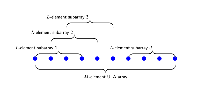
where the arrival vectors are equal to the original arrival vectors but multiplied by a direction-dependent phase shift. When you translate the original array J –1 more times, you get J copies of the array. If you form a single array from all these copies, then the length of the single array is M = L + (J – 1).
In practice, you start with an M-element array and form J overlapping subarrays. The number of elements in each subarray is L = M – J + 1. The following figure shows the relationship between the overall length of the array, M, the number of subarrays, J, and the length of each subarray, L.
For the pth subarray, the source signal arrival matrix is
The original arrival vector matrix is postmultiplied by a diagonal phase matrix.
The last step is averaging the signal covariance matrices over all J subarrays to form the averaged signal covariance matrix, Ravgs. The average signal covariance matrix depends on the smoothed source covariance matrix, Rsmooth.
You can show that the diagonal elements of the smoothed source covariance matrix are the same as the diagonal elements of the original source covariance matrix.
However, the off-diagonal elements are reduced. The reduction factor is the beam pattern of a J-element array.
In summary, you can reduce the degrading effect of source correlation by forming subarrays and using the smoothed covariance matrix as input to the MUSIC algorithm. Because of the beam pattern, larger angular separation of sources leads to reduced correlation.
Spatial smoothing for linear arrays is easily extended to 2D and 3D uniform arrays.