Multi-Hop Satellite Communications Link Between Two Ground Stations

This example demonstrates how to set up a multi-hop satellite communications link between two ground stations. The first ground station is located in India (Ground Station 1), and the second ground station is located in Australia (Ground Station 2). The link is routed via two satellites (Satellite 1 and Satellite 2). Each satellite acts as a regenerative repeater. A regenerative repeater receives an incoming signal, and then demodulates, remodulates, amplifies, and retransmits the received signal. The times over the course of a day during which Ground Station 1 can send data to Ground Station 2 are determined.

Create Satellite Scenario

Use satelliteScenario to create a satellite scenario. Use datetime to define the start time and stop time of the scenario. Set the sample time to 60 seconds.

startTime = datetime(2020,8,19,20,55,0);              % 19 August 2020 8:55 PM UTC
stopTime = startTime + days(1);                       % 20 August 2020 8:55 PM UTC
sampleTime = 60;                                      % seconds
sc = satelliteScenario(startTime,stopTime,sampleTime);

Launch Satellite Scenario Viewer

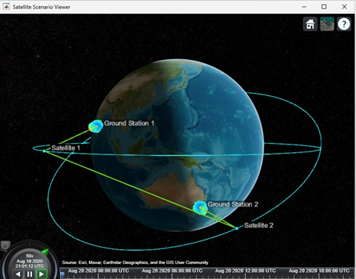
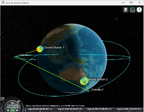
Use satelliteScenarioViewer to launch a Satellite Scenario Viewer.

satelliteScenarioViewer(sc);

Add the Satellites

Use satellite to add Satellite 1 and Satellite 2 to the scenario by specifying their Keplerian orbital elements corresponding to the scenario start time.

semiMajorAxis = 10000000;                  % meters
eccentricity = 0;
inclination = 0;                           % degrees
rightAscensionOfAscendingNode = 0;         % degrees
argumentOfPeriapsis = 0;                   % degrees
trueAnomaly = 0;                           % degrees
sat1 = satellite(sc, ...
    semiMajorAxis, ...
    eccentricity, ...
    inclination, ...
    rightAscensionOfAscendingNode, ...
    argumentOfPeriapsis, ...
    trueAnomaly, ...
    "Name","Satellite 1", ...
    "OrbitPropagator","two-body-keplerian");

semiMajorAxis = 10000000;                  % meters
eccentricity = 0;
inclination = 30;                          % degrees
rightAscensionOfAscendingNode = 120;       % degrees
argumentOfPeriapsis = 0;                   % degrees
trueAnomaly = 300;                         % degrees
sat2 = satellite(sc, ...
    semiMajorAxis, ...
    eccentricity, ...
    inclination, ...
    rightAscensionOfAscendingNode, ...
    argumentOfPeriapsis, ...
    trueAnomaly, ...
    "Name","Satellite 2", ...
    "OrbitPropagator","two-body-keplerian");

Add Gimbals to the Satellites

Use gimbal to add gimbals to the satellites. Each satellite consists of two gimbals on opposite sides of the satellite. One gimbal holds the receiver antenna and the other gimbal holds the transmitter antenna. The mounting location is specified in cartesian coordinates in the body frame of the satellite, which is defined by $$({\underset{}{\overset{ˆ}{x}}}_S,{\underset{}{\overset{ˆ}{y}}}_S,{\underset{}{\overset{ˆ}{z}}}_S)$$, where $${\underset{}{\overset{ˆ}{x}}}_S$$, $${\underset{}{\overset{ˆ}{y}}}_S$$ and $${\underset{}{\overset{ˆ}{z}}}_S$$ are the roll, pitch and yaw axes respectively, of the satellite. The mounting location of the gimbal that holds the receiver is $$-{\underset{}{\overset{ˆ}{y}}}_S+2{\underset{}{\overset{ˆ}{z}}}_S$$ meters and that of the gimbal that holds the transmitter is $${\underset{}{\overset{ˆ}{y}}}_S+2{\underset{}{\overset{ˆ}{z}}}_S$$ meters, as illustrated in the diagram below.

gimbalSat1Tx = gimbal(sat1, ...
    "MountingLocation",[0;1;2]);  % meters
gimbalSat2Tx = gimbal(sat2, ...
    "MountingLocation",[0;1;2]);  % meters
gimbalSat1Rx = gimbal(sat1, ...
    "MountingLocation",[0;-1;2]); % meters
gimbalSat2Rx = gimbal(sat2, ...
    "MountingLocation",[0;-1;2]); % meters

Add Receivers and Transmitters to the Gimbals

Each satellite consists of a receiver and a transmitter, constituting a regenerative repeater. Use receiver to add a receiver to the gimbals gimbalSat1Rx and gimbalSat2Rx. The mounting location of the receiving antenna with respect to the gimbal is $${\underset{}{\overset{ˆ}{z}}}_G$$ meters, as illustrated in the diagram above. The receiver gain to noise temperature ratio is 3dB/K and the required Eb/No is 4 dB.

sat1Rx = receiver(gimbalSat1Rx, ...
    "MountingLocation",[0;0;1], ...      % meters
    "GainToNoiseTemperatureRatio",3, ... % decibels/Kelvin
    "RequiredEbNo",4);                   % decibels
sat2Rx = receiver(gimbalSat2Rx, ...
    "MountingLocation",[0;0;1], ...      % meters
    "GainToNoiseTemperatureRatio",3, ... % decibels/Kelvin
    "RequiredEbNo",4);                   % decibels

Use gaussianAntenna to set the dish diameter of the receiver antennas on the satellites to 0.5 m. A Gaussian antenna has a radiation pattern that peaks at its boresight and decays radial-symmetrically based on a Gaussian distribution while moving away from boresight, as shown in the diagram below. The peak gain is a function of the dish diameter and aperture efficiency.

gaussianAntenna(sat1Rx, ...
    "DishDiameter",0.5);    % meters
gaussianAntenna(sat2Rx, ...
    "DishDiameter",0.5);    % meters

Use transmitter to add a transmitter to the gimbals gimbalSat1Tx and gimbalSat2Tx. The mounting location of the transmitting antenna with respect to the gimbal is $${\underset{}{\overset{ˆ}{z}}}_G$$ meters, where $$({\underset{}{\overset{ˆ}{x}}}_G,{\underset{}{\overset{ˆ}{y}}}_G,{\underset{}{\overset{ˆ}{z}}}_G)$$ define the body frame of the gimbal. The boresight of the antenna is aligned with $${\underset{}{\overset{ˆ}{z}}}_G$$. Both satellites transmit with a power of 15 dBW. The transmitter onboard Satellite 1 is used in the crosslink for sending data to Satellite 2 at a frequency of 30 GHz. The transmitter onboard Satellite 2 is used in the downlink to Ground Station 2 at a frequency of 27 GHz.

sat1Tx = transmitter(gimbalSat1Tx, ...
    "MountingLocation",[0;0;1], ...   % meters
    "Frequency",30e9, ...             % hertz
    "Power",15);                      % decibel watts
sat2Tx = transmitter(gimbalSat2Tx, ...
    "MountingLocation",[0;0;1], ...   % meters
    "Frequency",27e9, ...             % hertz
    "Power",15);                      % decibel watts

Like the receiver, the transmitter also uses a Gaussian antenna. Set the dish diameter of the transmitter antennas of the satellites to 0.5 m.

gaussianAntenna(sat1Tx, ...
    "DishDiameter",0.5);    % meters
gaussianAntenna(sat2Tx, ...
    "DishDiameter",0.5);    % meters

Add the Ground Stations

Use groundStation to add the ground stations at India (Ground Station 1) and Australia (Ground Station 2).

latitude = 12.9436963;          % degrees
longitude = 77.6906568;         % degrees
gs1 = groundStation(sc, ...
    latitude, ...
    longitude, ...
    "Name","Ground Station 1");

latitude = -33.7974039;        % degrees
longitude = 151.1768208;       % degrees
gs2 = groundStation(sc, ...
    latitude, ...
    longitude, ...
    "Name","Ground Station 2");

Add Gimbal to Each Ground Station

Use gimbal to add a gimbal to Ground Station 1 and Ground Station 2. The gimbal at Ground Station 1 holds a transmitter, and the gimbal at Ground Station 2 holds a receiver. The gimbals are located 5 meters above their respective ground stations, as illustrated in the diagram below. Consequently, their mounting locations are $$-5{\underset{}{\overset{ˆ}{z}}}_{GS}$$ meters, where $$({\underset{}{\overset{ˆ}{x}}}_{GS},{\underset{}{\overset{ˆ}{y}}}_{GS},{\underset{}{\overset{ˆ}{z}}}_{GS})$$ define the body axis of the ground stations. $${\underset{}{\overset{ˆ}{x}}}_{GS}$$, $${\underset{}{\overset{ˆ}{y}}}_{GS}$$ and $${\underset{}{\overset{ˆ}{z}}}_{GS}$$ always point North, East and down respectively. Therefore, the $${\underset{}{\overset{ˆ}{z}}}_{GS}$$ component of the gimbals is -5 meters so that they are placed above the ground station and not below. Furthermore, by default, the mounting angles of the gimbal are such that their body axes $$({\underset{}{\overset{ˆ}{x}}}_G,{\underset{}{\overset{ˆ}{y}}}_G,{\underset{}{\overset{ˆ}{z}}}_G)$$ are aligned with the parent (in this case, the ground station) body axes $$({\underset{}{\overset{ˆ}{x}}}_{GS},{\underset{}{\overset{ˆ}{y}}}_{GS},{\underset{}{\overset{ˆ}{z}}}_{GS})$$. As a result, when the gimbals are not steered, their $${\underset{}{\overset{ˆ}{z}}}_G$$ axis points straight down, and so does the antenna attached to it using default mounting angles as well. Therefore, you must set the mounting pitch angle to 180 degrees, so that $${\underset{}{\overset{ˆ}{z}}}_G$$ points straight up when the gimbal is not steered.

gimbalGs1 = gimbal(gs1, ...
    "MountingAngles",[0;180;0], ... % degrees
    "MountingLocation",[0;0;-5]);   % meters
gimbalGs2 = gimbal(gs2, ...
    "MountingAngles",[0;180;0], ... % degrees
    "MountingLocation",[0;0;-5]);   % meters

Add Transmitters and Receivers to Ground Station Gimbals

Use transmitter to add a transmitter to the gimbal at Ground Station 1. The uplink transmitter sends data to Satellite 1 at a frequency of 30 GHz and a power of 30 dBW. The transmitter antenna is mounted at $${\underset{}{\overset{ˆ}{z}}}_G$$ meters with respect to the gimbal.

gs1Tx = transmitter(gimbalGs1, ...
    "Name","Ground Station 1 Transmitter", ...
    "MountingLocation",[0;0;1], ...           % meters
    "Frequency",30e9, ...                     % hertz
    "Power",30);                              % decibel watts

Use gaussianAntenna to set the dish diameter of the transmitter antenna to 2 m.

gaussianAntenna(gs1Tx, ...
    "DishDiameter",2); % meters

Use receiver to add a receiver to the gimbal at Ground Station 2 to receive downlink data from Satellite 2. The receiver gain to noise temperature ratio is 3 dB/K and the required Eb/No is 1 dB. The mounting location of the receiver antenna is $${\underset{}{\overset{ˆ}{z}}}_G$$ meters with respect to the gimbal.

gs2Rx = receiver(gimbalGs2, ...
    "Name","Ground Station 2 Receiver", ...
    "MountingLocation",[0;0;1], ...        % meters
    "GainToNoiseTemperatureRatio",3, ...   % decibels/Kelvin
    "RequiredEbNo",1);                     % decibels

Use gaussianAntenna to set the dish diameter of the receiver antenna to 2 m.

gaussianAntenna(gs2Rx, ...
    "DishDiameter",2); % meters

Set Tracking Targets for Gimbals

For the best link quality, the antennas must continuously point at their respective targets. The gimbals can be steered independent of their parents (satellite or ground station), and configured to track other satellites and ground stations. Use pointAt to set the tracking target for the gimbals so that:

• The transmitter antenna at Ground Station 1 points at Satellite 1

• The receiver antenna aboard Satellite 1 points at Ground Station 1

• The transmitter antenna aboard Satellite 1 points at Satellite 2

• The receiver antenna aboard Satellite 2 points at Satellite 1

• The transmitter antenna aboard Satellite 2 points at Ground Station 2

• The receiver antenna at Ground Station 2 points at Satellite 2

pointAt(gimbalGs1,sat1);
pointAt(gimbalSat1Rx,gs1);
pointAt(gimbalSat1Tx,sat2);
pointAt(gimbalSat2Rx,sat1);
pointAt(gimbalSat2Tx,gs2);
pointAt(gimbalGs2,sat2);

When a target for a gimbal is set, its $${\underset{}{\overset{ˆ}{z}}}_G$$ axis will track the target. Since the antenna is on $${\underset{}{\overset{ˆ}{z}}}_G$$ and its boresight is aligned with $${\underset{}{\overset{ˆ}{z}}}_G$$, the antenna will also track the desired target.

Add Link Analysis and Visualize Scenario

Use link to add link analysis to the transmitter at Ground Station 1. The link is of regenerative repeater-type that originates at gs1Tx and ends at gs2Rx, and is routed via sat1Rx, sat1Tx, sat2Rx and sat2Tx.

lnk = link(gs1Tx,sat1Rx,sat1Tx,sat2Rx,sat2Tx,gs2Rx);

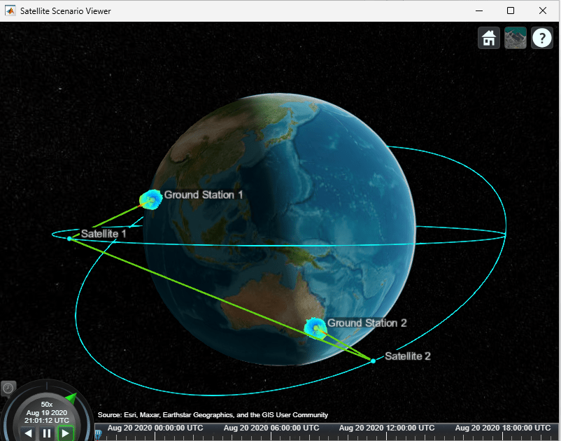
The Satellite Scenario Viewer automatically updates to display the entire scenario. Use the viewer as a visual confirmation that the scenario has been set up correctly. The green lines represent the link and confirm that the link is closed.

Determine Times When Link is Closed and Visualize Link Closures

Use the linkIntervals method to determine the times when the link is closed. The linkIntervals method outputs a table of the start and stop times of link closures that represent the intervals during which Ground Station 1 can send data to Ground Station 2. Source and Target are the first and last nodes in the link. If one of Source or Target is on a satellite, StartOrbit and EndOrbit provide the orbit count of the source or target satellite that they are attached directly or via gimbals, starting from the scenario start time. If both Source and Target are attached to a satellite, StartOrbit and EndOrbit provide the orbit count of the satellite to which Source is attached. Since both Source and Target are attached to ground stations, StartOrbit and EndOrbit are NaN.

linkIntervals(lnk)

ans=6×8 table
                Source                          Target               IntervalNumber         StartTime                EndTime           Duration    StartOrbit    EndOrbit
    ______________________________    ___________________________    ______________    ____________________    ____________________    ________    __________    ________

    "Ground Station 1 Transmitter"    "Ground Station 2 Receiver"          1           19-Aug-2020 20:55:00    19-Aug-2020 21:20:00      1500         NaN          NaN   
    "Ground Station 1 Transmitter"    "Ground Station 2 Receiver"          2           19-Aug-2020 23:38:00    20-Aug-2020 00:21:00      2580         NaN          NaN   
    "Ground Station 1 Transmitter"    "Ground Station 2 Receiver"          3           20-Aug-2020 09:34:00    20-Aug-2020 09:50:00       960         NaN          NaN   
    "Ground Station 1 Transmitter"    "Ground Station 2 Receiver"          4           20-Aug-2020 12:26:00    20-Aug-2020 12:58:00      1920         NaN          NaN   
    "Ground Station 1 Transmitter"    "Ground Station 2 Receiver"          5           20-Aug-2020 15:25:00    20-Aug-2020 16:05:00      2400         NaN          NaN   
    "Ground Station 1 Transmitter"    "Ground Station 2 Receiver"          6           20-Aug-2020 18:28:00    20-Aug-2020 19:13:00      2700         NaN          NaN   

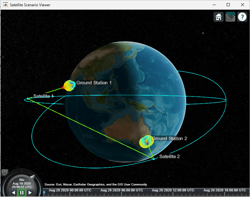
Use play to visualize the scenario simulation from its start time to stop time. The green lines disappear whenever the link cannot be closed.

play(sc);

Plot Link Margin at Ground Station 2

The link margin at a receiver is the difference between the energy per bit to noise power spectral density ratio (Eb/No) at the receiver and its RequiredEbNo. For successful link closure, the link margin must be positive at all receiver nodes. Higher the link margin, better the link quality. To calculate the link margin at final node, that is, Ground Station 2 Receiver, use ebno to get the Eb/No history at the Ground Station 2 Receiver, and subtract its RequiredEbNo from this quantity to get the link margin. Also, use plot to plot the calculate link margin.

[e, time] = ebno(lnk);
margin = e - gs2Rx.RequiredEbNo;
plot(time,margin,"LineWidth",2);
xlabel("Time");
ylabel("Link Margin (dB)");
grid on;

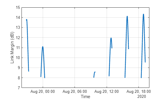
The gaps in the plot imply that the link was broken before reaching the final node in the link, or the line of sight between final node and the node before it, that is, Satellite 2, was broken. At all other times, the link margin is positive. This implies that Satellite 2 Transmitter power and Ground Station 2 Receiver sensitivity are always sufficient. It also implies that the margin is positive at all other hops of the link.

Modify Required Eb/No and Observe Effect on Link Intervals

Increase the RequiredEbNo of the receiver at Ground Station 2 from 1 dB to 10 dB and recompute the link intervals. Increasing RequiredEbNo essentially reduces the sensitivity of Ground Station 2 Receiver. This negatively impacts the resultant link closure times. The number of closed link intervals drops from six to five, and the duration of the closed link intervals is shorter.

gs2Rx.RequiredEbNo = 10; % decibels
linkIntervals(lnk)

ans=5×8 table
                Source                          Target               IntervalNumber         StartTime                EndTime           Duration    StartOrbit    EndOrbit
    ______________________________    ___________________________    ______________    ____________________    ____________________    ________    __________    ________

    "Ground Station 1 Transmitter"    "Ground Station 2 Receiver"          1           19-Aug-2020 20:55:00    19-Aug-2020 21:18:00      1380         NaN          NaN   
    "Ground Station 1 Transmitter"    "Ground Station 2 Receiver"          2           19-Aug-2020 23:43:00    20-Aug-2020 00:15:00      1920         NaN          NaN   
    "Ground Station 1 Transmitter"    "Ground Station 2 Receiver"          3           20-Aug-2020 12:30:00    20-Aug-2020 12:58:00      1680         NaN          NaN   
    "Ground Station 1 Transmitter"    "Ground Station 2 Receiver"          4           20-Aug-2020 15:29:00    20-Aug-2020 16:05:00      2160         NaN          NaN   
    "Ground Station 1 Transmitter"    "Ground Station 2 Receiver"          5           20-Aug-2020 18:32:00    20-Aug-2020 19:13:00      2460         NaN          NaN   

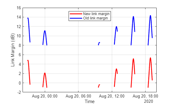
Additionally, the increase in RequiredEbNo negatively impacts the link margin. To observe this, recompute and plot the new link margin, and compare it with the previous plot. The link margin has reduced in general, implying that the link quality has gone down as a result of reducing the sensitivity of the receiver by increasing RequiredEbNo. At certain instances, the link margin is negative, signifying that there are times when the link does get broken at Ground Station 2 Receiver, even if it has line of sight to Satellite 2. This implies that the link closure is sometimes limited by the link margin, as opposed to just the line of sight between adjacent nodes.

[e, newTime] = ebno(lnk);
newMargin = e - gs2Rx.RequiredEbNo;
plot(newTime,newMargin,"r",time,margin,"b","LineWidth",2);
xlabel("Time");
ylabel("Link Margin (dB)");
legend("New link margin","Old link margin","Location","north");
grid on;

Next Steps

This example demonstrated how to set up a multi-hop regenerative repeater-type link and how to determine the times when the link is closed. The link closure times are influenced by the link margin at each receiver in the link. The link margin is the difference between energy per bit to noise power spectral density ratio (Eb/No) at the receiver and the required Eb/No. The Eb/No at a receiver is a function of:

• Orbit and pointing mode of satellites holding the transmitters and receivers

• Position of ground stations holding the transmitters and receivers

• Position, orientation, and pointing mode of the gimbals holding the transmitters and receivers

• Position and orientation of the transmitters and receivers with respect to their parents

• Specifications of the transmitters - power, frequency, bit rate, and system loss

• Specifications of the receivers - gain to noise temperature ratio, required Eb/No, and system loss

• Specifications of the transmitter and receiver antennas, such as dish diameter and aperture efficiency for a Gaussian antenna

Modify the above parameters and observe their impact on the link to perform different types of what-if analyses.