cgsl_0201: Redundant Unit Delay and Memory blocks
| ID: Title | cgsl_0201: Redundant Unit Delay and Memory blocks | ||
|---|---|---|---|
| Description | When preparing a model for code generation, | ||
| A | Remove redundant Unit Delay and Memory blocks. | ||
| Rationale | A | Redundant Unit Delay and Memory blocks use additional global memory. Removing the redundancies from a model reduces memory usage without impacting model behavior. | |
| Last Changed | R2013a | ||
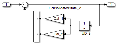
| Example | Recommended: Consolidated Unit Delays
void Reduced(void)
{
  ConsolidatedState_2 = Matrix_UD_Test - (Cal_1 * DWork.UD_3_DSTATE + Cal_2 *
    DWork.UD_3_DSTATE);
  DWork.UD_3_DSTATE = ConsolidatedState_2;
} | ||
Not Recommended: Redundant Unit Delays
void Redundant(void)
{
  RedundantState = (Matrix_UD_Test - Cal_2 * DWork.UD_1B_DSTATE) - Cal_1 *
    DWork.UD_1A_DSTATE;
  DWork.UD_1B_DSTATE = RedundantState;
  DWork.UD_1A_DSTATE = RedundantState;
} | |||
Unit Delay and Memory blocks exhibit commutative and distributive algebraic properties. When the blocks are part of an equation with one driving signal, you can move the Unit Delay and Memory blocks to a new position in the equation without changing the result.
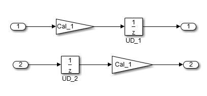
For the top path in the preceding example, the equations for the blocks are:
For the bottom path, the equations are:
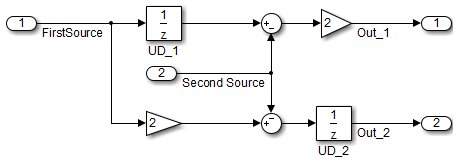
In contrast, if you add a secondary signal to the equations, the location of the Unit Delay block impacts the result. As the following example shows, the location of the Unit Delay block impacts the results due to the skewing of the time sample between the top and bottom paths.
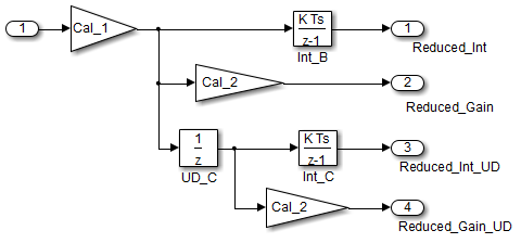
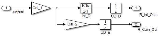
In cases with a single source and multiple destinations, the comparison is more complex. For example, in the following model, you can refactor the two Unit Delay blocks into a single unit delay.
From a black box perspective, the two models are equivalent. However, from a memory and computation perspective, differences exist between the two models. {
real_T rtb_Gain4;
rtb_Gain4 = Cal_1 * Redundant;
Y.Redundant_Gain = Cal_2 * rtb_Gain4;
Y.Redundant_Int = DWork.Int_A;
Y.Redundant_Int_UD = DWork.UD_A;
Y.Redundant_Gain_UD = DWork.UD_B;
DWork.Int_A = 0.01 * rtb_Gain4 + DWork.Int_A;
DWork.UD_A = Y.Redundant_Int;
DWork.UD_B = Y.Redundant_Gain;
}{
real_T rtb_Gain1;
real_T rtb_UD_C;
rtb_Gain1 = Cal_1 * Reduced;
rtb_UD_C = DWork.UD_C;
Y.Reduced_Gain_UD = Cal_2 * DWork.UD_C;
Y.Reduced_Gain = Cal_2 * rtb_Gain1;
Y.Reduced_Int = DWork.Int_B;
Y.Reduced_Int_UD = DWork.Int_C;
DWork.UD_C = rtb_Gain1;
DWork.Int_B = 0.01 * rtb_Gain1 + DWork.Int_B;
DWork.Int_C = 0.01 * rtb_UD_C + DWork.Int_C;
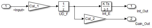
}In this case, the original model is more efficient. In the first code example, there are three global variables, two from the Unit Delay blocks (DWork.UD_A and DWork.UD_B) and one from the discrete time integrator (DWork.Int_A). The second code example shows a reduction to one global variable generated by the unit delays (Dwork.UD_C), but there are two global variables due to the redundant Discrete Time Integrator blocks (DWork.Int_B and DWork.Int_C). The Discrete Time Integrator block path introduces an additional local variable (rtb_UD_C) and two additional computations. By contrast, the refactored model (second) below is more efficient.
{
  real_T rtb_Gain4_f:
  real_T rtb_Int_D;
  rtb_Gain4_f = Cal_1 * U.Input;
  rtb_Int_D = DWork.Int_D;
  Y.R_Int_Out = DWork.UD_D;
  Y.R_Gain_Out = DWork.UD_E;
  DWork.Int_D = 0.01 * rtb_Gain4_f + DWork.Int_D;
  DWork.UD_D = rtb_Int_D;
  DWork.UD_E = Cal_2 * rtb_Gain4_f;
}
{
real_T rtb_UD_F;
rtb_UD_F = DWork.UD_F;
Y.Gain_Out = Cal_2 * DWork.UD_F;
Y.Int_Out = DWork.Int_E;
DWork.UD_F = Cal_1 * U.Input;
DWork.Int_E = 0.01 * rtb_UD_F + DWork.Int_E;
}The code for the refactored model is more efficient because the branches from the root signal do not have a redundant unit delay. | |||