fairnessWeights
Syntax
Description
weights = fairnessWeights(Tbl,AttributeName,ResponseVarName)AttributeName sensitive attribute and
the ResponseVarName response variable in the data set
Tbl. For every combination of a group in the sensitive attribute and
a class label in the response variable, the software computes a weight value. The function
then assigns each observation in Tbl its corresponding weight. The
returned weights vector introduces fairness across the sensitive
attribute groups. For more information, see Algorithms.
weights = fairnessWeights(Tbl,AttributeName,Y)Y.
weights = fairnessWeights(___,Weights=initialWeights)initialWeights before
computing the fairness weights, using any of the input argument combinations in previous
syntaxes. These initial weights are typically used to capture some aspect of the data set
that is unrelated to the sensitive attribute, such as expected class distributions.
Examples
Compute fairness weights. Then, compare the fairness weights to the default observation weights using grouped scatter plots.
Suppose you want to create a binary classifier that predicts whether a patient is a smoker based on the patient's diastolic and systolic blood pressure values. Furthermore, you want the model predictions to be independent of the gender of the patient. Before training the model, you can use fairness weights to try to reduce the effects of gender status on the smoker status predictions.
Load the patients data set, which contains medical information for 100 patients. Convert the Gender and Smoker variables to categorical variables. Specify the descriptive category names Smoker and Nonsmoker rather than 1 and 0.
load patients
Gender = categorical(Gender);
Smoker = categorical(Smoker,logical([1 0]), ...
    ["Smoker","Nonsmoker"]);
Create a table using the Gender and Smoker variables in addition to the Diastolic and Systolic variables.
tbl = table(Diastolic,Gender,Smoker,Systolic)
tbl=100×4 table
    Diastolic    Gender     Smoker      Systolic
    _________    ______    _________    ________

       93        Male      Smoker         124
       77        Male      Nonsmoker      109
       83        Female    Nonsmoker      125
       75        Female    Nonsmoker      117
       80        Female    Nonsmoker      122
       70        Female    Nonsmoker      121
       88        Female    Smoker         130
       82        Male      Nonsmoker      115
       78        Male      Nonsmoker      115
       86        Female    Nonsmoker      118
       77        Female    Nonsmoker      114
       68        Female    Nonsmoker      115
       74        Male      Nonsmoker      127
       95        Male      Smoker         130
       79        Female    Nonsmoker      114
       92        Male      Smoker         130
      ⋮
Compute fairness weights with respect to the sensitive attribute Gender and the binary response variable Smoker, and add the fairness weights to tbl.
fairWeights = fairnessWeights(tbl,"Gender","Smoker");
tbl.Weights = fairWeights;
Display the fairness weight for each combination of gender and smoker status.
tblstats = grpstats(tbl,["Gender","Smoker"],@(x)unique(x), ...
    DataVars="Weights", ...
    VarNames=["Gender","Smoker","NumObservations","FairnessWeight"])
tblstats=4×4 table
                        Gender     Smoker      NumObservations    FairnessWeight
                        ______    _________    _______________    ______________

    Female_Smoker       Female    Smoker             13               1.3862
    Female_Nonsmoker    Female    Nonsmoker          40               0.8745
    Male_Smoker         Male      Smoker             21              0.76095
    Male_Nonsmoker      Male      Nonsmoker          26               1.1931
You can replicate the fairness weight computation by using the tblstats output. For example, compute the fairness weight directly for the group of female smokers.
numSmoker = sum(tblstats.NumObservations([1 3]));
numTotal = sum(tblstats.NumObservations);
numFemale = sum(tblstats.NumObservations([1 2]));
numFemaleSmoker = tblstats.NumObservations(1);

pIdealFemaleSmoker = (numSmoker/numTotal)*(numFemale/numTotal)
pIdealFemaleSmoker =
0.1802
pObservedFemaleSmoker = numFemaleSmoker/numTotal
pObservedFemaleSmoker =
0.1300
weightFemaleSmoker = pIdealFemaleSmoker/pObservedFemaleSmoker
weightFemaleSmoker =
1.3862
For this group, the ideal probability pIdealFemaleSmoker is greater than the observed probability pObservedFemaleSmoker. This result indicates bias against the smoker class for female patients in the original data set.
Visualize the fairness weights using grouped scatter plots. Without the fairness weights, all observations have the same weight by default.
markSize = 20;

tiledlayout(1,2)
nexttile
gscatter(Diastolic,Systolic,Gender.*Smoker,[],[], ...
    markSize)
legend(Location="southoutside")
title("Original Observations")
nexttile
gscatter(Diastolic,Systolic,Gender.*Smoker,[],[], ...
    markSize*tblstats.FairnessWeight)
legend(Location="southoutside")
title("Weighted Observations")
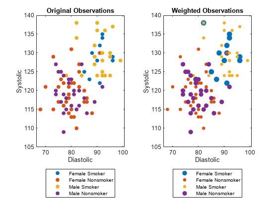
In the weighted scheme, the female smoker and male nonsmoker observations have more weight than in the original scheme.
To understand how fairness weights affect the observations, find the statistical parity difference (SPD) for each group in Gender after applying the fairness weights. Use the fairnessMetrics function, which computes bias and group metrics for a data set or binary classification model with respect to sensitive attributes.
metrics = fairnessMetrics(tbl,"Smoker", ...
    SensitiveAttributeNames="Gender",Weights="Weights");
metrics.PositiveClass
ans = categorical
     Nonsmoker
report(metrics,BiasMetrics="StatisticalParityDifference")ans=2×3 table
SensitiveAttributeNames Groups StatisticalParityDifference
_______________________ ______ ___________________________
Gender Female 0
Gender Male -6.6613e-16
The SPD for each group in the sensitive attribute is approximately 0. This result indicates that, with the fairness weights, the proportion of female nonsmokers to female patients is the same as the proportion of male nonsmokers to male patients.
You can now use the fairness weights to train a binary classifier. For example, train a tree classifier.
tree = fitctree(tbl,"Smoker",Weights="Weights")
tree =
  ClassificationTree
           PredictorNames: {'Diastolic'  'Gender'  'Systolic'}
             ResponseName: 'Smoker'
    CategoricalPredictors: 2
               ClassNames: [Smoker    Nonsmoker]
           ScoreTransform: 'none'
          NumObservations: 100


  Properties, Methods
See how predictions change when you train a binary classifier with fairness weights. In particular, compare the disparate impact and accuracy of the predictions.
Load the sample data census1994, which contains the training data adultdata and the test data adulttest. The data sets consist of demographic information from the US Census Bureau that can be used to predict whether an individual makes over $50,000 per year. Preview the first few rows of the training data set.
load census1994
head(adultdata)
age workClass fnlwgt education education_num marital_status occupation relationship race sex capital_gain capital_loss hours_per_week native_country salary
___ ________________ __________ _________ _____________ _____________________ _________________ _____________ _____ ______ ____________ ____________ ______________ ______________ ______
39 State-gov 77516 Bachelors 13 Never-married Adm-clerical Not-in-family White Male 2174 0 40 United-States <=50K
50 Self-emp-not-inc 83311 Bachelors 13 Married-civ-spouse Exec-managerial Husband White Male 0 0 13 United-States <=50K
38 Private 2.1565e+05 HS-grad 9 Divorced Handlers-cleaners Not-in-family White Male 0 0 40 United-States <=50K
53 Private 2.3472e+05 11th 7 Married-civ-spouse Handlers-cleaners Husband Black Male 0 0 40 United-States <=50K
28 Private 3.3841e+05 Bachelors 13 Married-civ-spouse Prof-specialty Wife Black Female 0 0 40 Cuba <=50K
37 Private 2.8458e+05 Masters 14 Married-civ-spouse Exec-managerial Wife White Female 0 0 40 United-States <=50K
49 Private 1.6019e+05 9th 5 Married-spouse-absent Other-service Not-in-family Black Female 0 0 16 Jamaica <=50K
52 Self-emp-not-inc 2.0964e+05 HS-grad 9 Married-civ-spouse Exec-managerial Husband White Male 0 0 45 United-States >50K
Each row contains the demographic information for one adult. The last column, salary, shows whether a person has a salary less than or equal to $50,000 per year or greater than $50,000 per year.
Remove observations from adultdata and adulttest that contain missing values.
adultdata = rmmissing(adultdata);
adulttest = rmmissing(adulttest);
Train a neural network classifier using the training set adultdata. Specify salary as the response variable and fnlwgt as the observation weights. Standardize the predictor variables before training the model. After training the model, predict the salary (class label) of the observations in the test set adulttest.
rng("default") % For reproducibility
mdl = fitcnet(adultdata,"salary",Weights="fnlwgt", ...
    Standardize=true);
labels = predict(mdl,adulttest);
Compute the fairness weights with respect to the sensitive attribute race. Use the initial observation weights fnlwgt to adjust the fairness weight computation. Create a new table newadultdata that contains the adjusted fairness weights rather than the initial observation weights.
fw = fairnessWeights(adultdata,"race","salary", ...
    Weights="fnlwgt");
newadultdata = adultdata;
newadultdata.fnlwgt = fw;
Train the same type of neural network classifier as mdl, but use the adjusted fairness weights. As before, predict the salary (class label) of the observations in the test set adulttest.
rng("default") % For reproducibility
newMdl = fitcnet(newadultdata,"salary",Weights="fnlwgt", ...
    Standardize=true);
newLabels = predict(newMdl,adulttest);
Compare the disparate impact values for the predictions made by the original model (mdl) to the predictions made by the model trained with fairness weights (newMdl). For each group in the sensitive attribute, the disparate impact is the proportion of predictions in that group with a positive class value () divided by the proportion of predictions in the reference group with a positive class value (). An ideal classifier makes predictions so that, for each group, is close to (that is, the disparate impact value is close to 1).
Compute the disparate impact values for the mdl predictions and the newMdl predictions by using the fairnessMetrics function. Specify to include observation weights. You can use the report object function to display bias metrics, such as disparate impact, that are stored in the metricsResults object.
metricsResults = fairnessMetrics(adulttest,"salary", ...
    SensitiveAttributeNames="race",Predictions=[labels,newLabels], ...
    Weights="fnlwgt",ModelNames=["Original Model","New Model"]);
metricsResults.PositiveClass
ans = categorical
     >50K
metricsResults.ReferenceGroup
ans =
'White'
report(metricsResults,BiasMetrics="DisparateImpact")ans=5×5 table
Metrics SensitiveAttributeNames Groups Original Model New Model
_______________ _______________________ __________________ ______________ _________
DisparateImpact race Amer-Indian-Eskimo 0.20508 0.46838
DisparateImpact race Asian-Pac-Islander 1.1012 1.2304
DisparateImpact race Black 0.44286 0.68301
DisparateImpact race Other 0.33739 0.74539
DisparateImpact race White 1 1
For the mdl predictions, several of the disparate impact values are well below 1, which indicates bias in the predictions with respect to the positive class >50K and the sensitive attribute race. Compared to the disparate impact values for the mdl predictions, most of the disparate impact values for the newMdl predictions are closer to 1.
Visually compare the disparate impact values by using a bar graph returned by the plot object function.
plot(metricsResults,"DisparateImpact")
legend(Location="southwest")
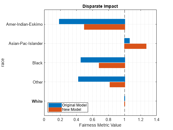
The fairness weights seem to improve the model predictions on the test set with respect to the disparate impact metric.
Check whether the fairness weights have negatively affected the accuracy of the model predictions. Compute the accuracy of the test set predictions for the two models mdl and newMdl.
accuracy = 1-loss(mdl,adulttest,"salary")accuracy = 0.8429
newAccuracy = 1-loss(newMdl,adulttest,"salary")newAccuracy = 0.8427
The model trained using fairness weights (newMdl) achieves similar test set accuracy compared to the model trained without fairness weights (mdl).
Input Arguments
Output Arguments
Algorithms
Assume x is an observation in class k with sensitive attribute
g. If you do not specify initial weights
(initialWeights), then the fairnessWeights
function assigns the following fairness weight to the observation: .
ng is the number of observations with sensitive attribute g.
nk is the number of observations in class k.
ngk is the number of observations in class k with sensitive attribute g.
n is the total number of observations.
is the ideal probability of an observation having sensitive attribute g and being in class k—that is, the product of the probability of an observation having sensitive attribute g and the probability of an observation being in class k. Note that this equation holds for the true probability if the sensitive attribute and the response variable are independent.
is the observed probability of an observation having sensitive attribute g and being in class k.
For more information, see [1].
If you specify initial weights, then the function computes fw(x) using the sum of the initial weights rather than the number of observations. For example, instead of using ng, the function uses the sum of the initial weights of the observations with sensitive attribute g.
References
[1] Kamiran, Faisal, and Toon Calders. “Data Preprocessing Techniques for Classification without Discrimination.” Knowledge and Information Systems 33, no. 1 (October 2012): 1–33. https://doi.org/10.1007/s10115-011-0463-8.
Version History
Introduced in R2022b