Fit a Generalized Linear Mixed-Effects Model
This example shows how to fit a generalized linear mixed-effects model (GLME) to sample data.
Load the Sample Data
Load the mfr sample data set.
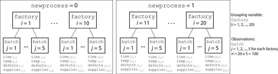
load mfr.matA manufacturing company operates 50 factories across the world, and each runs a batch process to create a finished product. The company wants to decrease the number of defects in each batch, so it developed a new manufacturing process. However, the company wants to test the new process in select factories to ensure that it is effective before rolling it out to all 50 locations.
To test whether the new process significantly reduces the number of defects in each batch, the company selected 20 of its factories at random to participate in an experiment. Ten factories implemented the new process, while the other ten used the old process.
In each of the 20 factories (i = 1, 2, ..., 20), the company ran five batches (j = 1, 2, ..., 5) and recorded the following data in the table mfr:
Flag to indicate use of the new process. If the batch used the new process, then
newprocess = 1. If the batch used the old process, thennewprocess = 0.Processing time for the batch, in hours (
time).Temperature of the batch, in degrees Celsius (
temp).Supplier of the chemical used in the batch (
supplier).supplieris a categorical variable with levelsA,B, andC, where each level represents one of the three suppliers.Number of defects in the batch (
defects).
The data also includes time_dev and temp_dev, which represent the absolute deviation of time and temperature, respectively, from the process standard of 3 hours and 20 degrees Celsius. The response variable defects has a Poisson distribution. This is simulated data.
The company wants to determine whether the new process significantly reduces the number of defects in each batch, while accounting for quality differences that might exist due to factory-specific variations in time, temperature, and supplier. The number of defects per batch can be modeled using a Poison distribution:
Use a generalized linear mixed-effects model to model the number of defects per batch:
,
where
is the number of defects observed in the batch produced by factory i during batch j.
is the mean number of defects corresponding to factory i (where i = 1, 2, ..., 20) during batch j (where j = 1, 2, ..., 5).
, , and are the measurements for each variable that correspond to factory i during batch j. For example, indicates whether the batch produced by factory i during batch j used the new process.
and are dummy variables that use effects (sum-to-zero) coding to indicate whether company
CorB, respectively, supplied the process chemicals for the batch produced by factory i during batch j.is a random-effects intercept for each factory i that accounts for factory-specific variation in quality.
Fit a GLME Model and Interpret the Results
Fit a generalized linear mixed-effects model using newprocess, time_dev, temp_dev, and supplier as fixed-effects predictors. Include a random-effects term for intercept grouped by factory, to account for quality differences that might exist due to factory-specific variations. The response variable defects has a Poisson distribution, and the appropriate link function for this model is log. Use the Laplace fit method to estimate the coefficients. Specify the dummy variable encoding as 'effects', so the dummy variable coefficients sum to 0.
glme = fitglme(mfr,...
'defects ~ 1 + newprocess + time_dev + temp_dev + supplier + (1|factory)',...
'Distribution','Poisson','Link','log','FitMethod','Laplace',...
'DummyVarCoding','effects')
glme =
Generalized linear mixed-effects model fit by ML

Model information:
    Number of observations             100
    Fixed effects coefficients           6
    Random effects coefficients         20
    Covariance parameters                1
    Distribution                    Poisson
    Link                            Log
    FitMethod                       Laplace

Formula:
    defects ~ 1 + newprocess + time_dev + temp_dev + supplier + (1 | factory)

Model fit statistics:
    AIC       BIC       LogLikelihood    Deviance
    416.35    434.58    -201.17          402.35

Fixed effects coefficients (95% CIs):
    Name                   Estimate     SE          tStat       DF    pValue        Lower        Upper
    {'(Intercept)'}           1.4689     0.15988      9.1875    94    9.8194e-15       1.1515       1.7864
    {'newprocess' }         -0.36766     0.17755     -2.0708    94      0.041122     -0.72019    -0.015134
    {'time_dev'   }        -0.094521     0.82849    -0.11409    94       0.90941      -1.7395       1.5505
    {'temp_dev'   }         -0.28317      0.9617    -0.29444    94       0.76907      -2.1926       1.6263
    {'supplier_C' }        -0.071868    0.078024     -0.9211    94       0.35936     -0.22679     0.083051
    {'supplier_B' }         0.071072     0.07739     0.91836    94       0.36078    -0.082588      0.22473

Random effects covariance parameters:
Group: factory (20 Levels)
    Name1                  Name2                  Type           Estimate
    {'(Intercept)'}        {'(Intercept)'}        {'std'}        0.31381

Group: Error
    Name                        Estimate
    {'sqrt(Dispersion)'}        1
The Model information table displays the total number of observations in the sample data (100), the number of fixed- and random-effects coefficients (6 and 20, respectively), and the number of covariance parameters (1). It also indicates that the response variable has a Poisson distribution, the link function is Log, and the fit method is Laplace.
Formula indicates the model specification using Wilkinson’s notation.
The Model fit statistics table displays statistics used to assess the goodness of fit of the model. This includes the Akaike information criterion (AIC), Bayesian information criterion (BIC) values, log likelihood (LogLikelihood), and deviance (Deviance) values.
The Fixed effects coefficients table indicates that fitglme returned 95% confidence intervals. It contains one row for each fixed-effects predictor, and each column contains statistics corresponding to that predictor. Column 1 (Name) contains the name of each fixed-effects coefficient, column 2 (Estimate) contains its estimated value, and column 3 (SE) contains the standard error of the coefficient. Column 4 (tStat) contains the t-statistic for a hypothesis test that the coefficient is equal to 0. Column 5 (DF) and column 6 (pValue) contain the degrees of freedom and p-value that correspond to the t-statistic, respectively. The last two columns (Lower and Upper) display the lower and upper limits, respectively, of the 95% confidence interval for each fixed-effects coefficient.
Random effects covariance parameters displays a table for each grouping variable (here, only factory), including its total number of levels (20), and the type and estimate of the covariance parameter. Here, std indicates that fitglme returns the standard deviation of the random effect associated with the factory predictor, which has an estimated value of 0.31381. It also displays a table containing the error parameter type (here, the square root of the dispersion parameter), and its estimated value of 1.
The standard display generated by fitglme does not provide confidence intervals for the random-effects parameters. To compute and display these values, use covarianceParameters.
Check Significance of Random Effect
To determine whether the random-effects intercept grouped by factory is statistically significant, compute the confidence intervals for the estimated covariance parameter.
[psi,dispersion,stats] = covarianceParameters(glme);
covarianceParameters returns the estimated covariance parameter in psi, the estimated dispersion parameter dispersion, and a cell array of related statistics stats. The first cell of stats contains statistics for factory, while the second cell contains statistics for the dispersion parameter.
Display the first cell of stats to see the confidence intervals for the estimated covariance parameter for factory.
stats{1}ans =
Covariance Type: Isotropic
Group Name1 Name2 Type Estimate Lower Upper
factory {'(Intercept)'} {'(Intercept)'} {'std'} 0.31381 0.19253 0.51148
The columns Lower and Upper display the default 95% confidence interval for the estimated covariance parameter for factory. Because the interval [0.19253,0.51148] does not contain 0, the random-effects intercept is significant at the 5% significance level. Therefore, the random effect due to factory-specific variation must be considered before drawing any conclusions about the effectiveness of the new manufacturing process.
Compare Two Models
Compare the mixed-effects model that includes a random-effects intercept grouped by factory with a model that does not include the random effect, to determine which model is a better fit for the data. Fit the first model, FEglme, using only the fixed-effects predictors newprocess, time_dev, temp_dev, and supplier. Fit the second model, glme, using these same fixed-effects predictors, but also including a random-effects intercept grouped by factory.
FEglme = fitglme(mfr,...
'defects ~ 1 + newprocess + time_dev + temp_dev + supplier',...
'Distribution','Poisson','Link','log','FitMethod','Laplace');

glme = fitglme(mfr,...
'defects ~ 1 + newprocess + time_dev + temp_dev + supplier + (1|factory)',...
'Distribution','Poisson','Link','log','FitMethod','Laplace');
Compare the two models using a likelihood ratio test. Specify 'CheckNesting' as true, so compare returns a warning if the nesting requirements are not satisfied.
results = compare(FEglme,glme,'CheckNesting',true)results =
Theoretical Likelihood Ratio Test
Model DF AIC BIC LogLik LRStat deltaDF pValue
FEglme 6 431.02 446.65 -209.51
glme 7 416.35 434.58 -201.17 16.672 1 4.4435e-05
compare returns the degrees of freedom (DF), the Akaike information criterion (AIC), Bayesian information criterion (BIC), and log likelihood values for each model. glme has smaller AIC, BIC, and log likelihood values than FEglme, which indicates that glme (the model containing the random-effects term for intercept grouped by factory) is the better-fitting model for this data. Additionally, the small p-value indicates that compare rejects the null hypothesis that the response vector was generated by the fixed-effects-only model FEglme, in favor of the alternative that the response vector was generated by the mixed-effects model glme.
Plot the Results
Generate the fitted conditional mean values for the model.
mufit = fitted(glme);
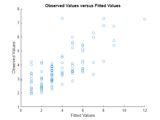
Plot the observed response values versus the fitted response values.
figure
scatter(mfr.defects,mufit)
title('Observed Values versus Fitted Values')
xlabel('Fitted Values')
ylabel('Observed Values')
Create diagnostic plots using conditional Pearson residuals to test model assumptions. Since raw residuals for generalized linear mixed-effects models do not have a constant variance across observations, use the conditional Pearson residuals instead.
Plot a histogram to visually confirm that the mean of the Pearson residuals is equal to 0. If the model is correct, we expect the Pearson residuals to be centered at 0.
plotResiduals(glme,'histogram','ResidualType','Pearson')
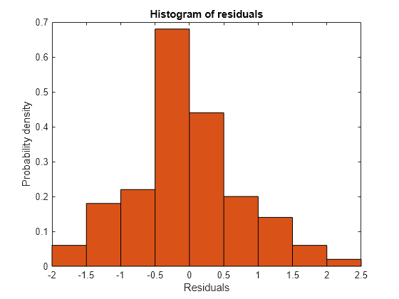
The histogram shows that the Pearson residuals are centered at 0.
Plot the Pearson residuals versus the fitted values, to check for signs of nonconstant variance among the residuals (heteroscedasticity). We expect the conditional Pearson residuals to have a constant variance. Therefore, a plot of conditional Pearson residuals versus conditional fitted values should not reveal any systematic dependence on the conditional fitted values.
plotResiduals(glme,'fitted','ResidualType','Pearson')
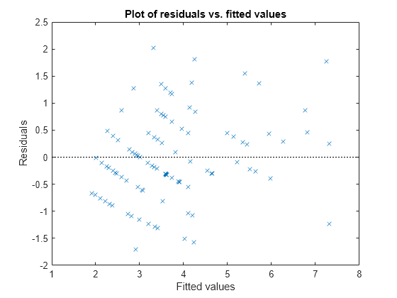
The plot does not show a systematic dependence on the fitted values, so there are no signs of nonconstant variance among the residuals.
Plot the Pearson residuals versus lagged residuals, to check for correlation among the residuals. The conditional independence assumption in GLME implies that the conditional Pearson residuals are approximately uncorrelated.
plotResiduals(glme,'lagged','ResidualType','Pearson')
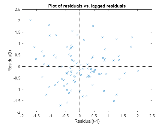
There is no pattern to the plot, so there are no signs of correlation among the residuals.
See Also
fitglme | GeneralizedLinearMixedModel