Lasso Regularization

This example shows how lasso identifies and discards unnecessary predictors.

Generate 200 samples of five-dimensional artificial data X from exponential distributions with various means.

rng(3,'twister') % For reproducibility
X = zeros(200,5);
for ii = 1:5
    X(:,ii) = exprnd(ii,200,1);
end

Generate response data Y = X * r + eps , where r has just two nonzero components, and the noise eps is normal with standard deviation 0.1.

r = [0;2;0;-3;0];
Y = X*r + randn(200,1)*.1;

Fit a cross-validated sequence of models with lasso , and plot the result.

[b,fitinfo] = lasso(X,Y,'CV',10);
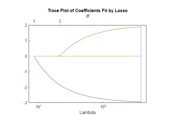
lassoPlot(b,fitinfo,'PlotType','Lambda','XScale','log');

The plot shows the nonzero coefficients in the regression for various values of the Lambda regularization parameter. Larger values of Lambda appear on the left side of the graph, meaning more regularization, resulting in fewer nonzero regression coefficients.

The dashed vertical lines represent the Lambda value with minimal mean squared error (on the right), and the Lambda value with minimal mean squared error plus one standard deviation. This latter value is a recommended setting for Lambda. These lines appear only when you perform cross validation. Cross validate by setting the 'CV' name-value pair argument. This example uses 10-fold cross validation.

The upper part of the plot shows the degrees of freedom (df), meaning the number of nonzero coefficients in the regression, as a function of Lambda. On the left, the large value of Lambda causes all but one coefficient to be 0. On the right all five coefficients are nonzero, though the plot shows only two clearly. The other three coefficients are so small that you cannot visually distinguish them from 0.

For small values of Lambda (toward the right in the plot), the coefficient values are close to the least-squares estimate.

Find the Lambda value of the minimal cross-validated mean squared error plus one standard deviation. Examine the MSE and coefficients of the fit at that Lambda.

lam = fitinfo.Index1SE;
fitinfo.MSE(lam)

ans = 
0.1398

b(:,lam)

ans = 5×1

         0
    1.8855
         0
   -2.9367
         0

lasso did a good job finding the coefficient vector r.

For comparison, find the least-squares estimate of r.

rhat = X\Y

rhat = 5×1

   -0.0038
    1.9952
    0.0014
   -2.9993
    0.0031

The estimate b(:,lam) has slightly more mean squared error than the mean squared error of rhat.

res = X*rhat - Y;     % Calculate residuals
MSEmin = res'*res/200 % b(:,lam) value is 0.1398

MSEmin = 
0.0088

But b(:,lam) has only two nonzero components, and therefore can provide better predictive estimates on new data.